Download
1 / 36
410 likes | 546 Views
Understand the importance of NPV estimates, scenario analysis, sensitivity analysis, and simulation in evaluating project viability. Learn to assess forecasting risks and explore managerial options in capital budgeting decisions.

E N D
Evaluating NPV Estimates Project Analysis and Evaluation Chapter 11 • NPV estimates are just that – estimates! • A positive NPV is a good start – but now we need to take a closer look • Forecasting risk – how sensitive is our NPV to changes in the cash flow estimates; the more sensitive, the greater the forecasting risk • Sources of value – why does this project create value?
Scenario Analysis( What-if Analysis ) • What happens to the NPV under different cash flow scenarios? • At the very least look at: • Best case – high revenues, low costs • Base Case – most likely range of possible outcomes. • Worst case – low revenues, high costs • Best case and worst case are not necessarily probable, but they can still be possible
Project Example • Consider the project discussed on page 346 to 347. • The initial cost is $200,000 and the project has a 5-year life. • There is no salvage. Depreciation is straight-line, the required return is 12%, and the tax rate is 34% • NPV of the base case is $15,567 • NPV best case is $159,504 • NPV of the worst case is -$111,719
Scenario Analysis Ranges of outcomes for each variable can be hypothesized Note:“Lower” ≠ Worst “Upper” ≠ Best (shaded)
CF = NI + DEP = 59,800 So, N = 5; I/Y = 12; PMT = 59,800; CPT PV = -215,565.62, Hence the Base Case NPV is 15,567
CF = NI + DEP = 99,730 So, N = 5; I/Y = 12; PMT = 99,730; CPT PV = -359,504.33, Hence the Best Case NPV is 159,504.33
CF = NI + DEP = 24,490 So, N = 5; I/Y = 12; PMT = 24,490; CPT PV = -88,280.97, Hence the Worst Case NPV is - 111,719
Problems with Scenario Analysis • Considers only a few possible out-comes • Assumes perfectly correlated inputs • All “bad” values occur together and all “good” values occur together • Focuses on stand-alone risk, although subjective adjustments can be made
Summary of Scenario AnalysisVaries Price, Quantity, and Cost Estimates
Sensitivity Analysis • What happens to NPV when we vary just one variable at a time • This is a subset of scenario analysis where we are looking at the effect of specific variableson NPV • The greater the volatility in NPV in relation to a specific variable, the larger the forecasting risk associated with that variable, and the more attention we want to pay to its estimation
Summary of Sensitivity Analysis Vary only Unit Salesfor this Sensitivity Analysis
Strengths of Sensitivity Analysis • It provides an indication of stand-alone risk. • It identifies dangerous variables. • It gives some breakeven information. Weaknesses of Sensitivity Analysis • But does not reflect diversification. • It says nothing about the likelihood of change in a variable. • It ignores relationships among variables.
Disadvantages of BothSensitivity and Scenario Analysis Neither provides a decision rule. • No indication whether a project’s expected return is sufficient to compensate for its risk. Both Ignore diversification. • Measures only stand-alone risk, which may not be the most relevant risk in capital budgeting.
Simulation Analysis • Simulation is really just an expanded sensitivity and scenario analysis • Monte Carlosimulation can estimate thousands of possible outcomes based on conditional probability distributions and constraints for each of the variables, such as a Nest Egg Calculator. • The output is a probability distribution for NPV with an estimate of the probability of obtaining a positive net present value • The simulation only works as well as the information that is entered and very bad decisions can be made if care is not taken to analyze the interaction between variables https://retirementplans.vanguard.com/VGApp/pe/pubeducation/calculators/RetirementNestEggCalc.jsf
Making A Decision • Beware of the “Paralysis of Analysis” • At some point you have to make a decision • If the majority of your scenarios have positive NPVs, then you can feel reasonably comfortable about accepting the project • If you have a crucial variable that leads to a negative NPV with a small change in the estimates, then you may want to forego the project
Managerial Options • Capital budgeting projects often provide other options that we have not yet considered • Contingency planning • Option to expand • Option to abandon • Option to wait • Strategic options (or Real Options) – say entry into the Chinese market
Capital Rationing • Capital rationing occurs when a firm or division has limited resources • Soft rationing – the limited resources are temporary or often self-imposed by management. • The profitability index is a useful tool when faced with soft rationing • Hard rationing – capital will never be available for this project
Quick Quiz • What is scenario analysis and why is it important? • What is sensitivity analysis and why is it important? • What are some additional managerial options that should be considered?
Breakeven Analysis Section 11.3 • The Operating (or CASH) Breakeven Point • Fixed Operating Costs • Variable Operating Costs • The Algebraic Approach uses the following variables P = Sale price per unit Q = Sales quantity in units FC = Fixed operating cost per period V = Variable operating cost per unit EBIT = (P x Q) - FC - (V x Q) = Q x (P - V) - FC • $ 0 = Q x (P - V) – FC FC Q = P-V
Example A firm has fixed operating costs of $2,500, a $10 sale price per unit, and a $5 per unit variable operating cost. Compute its operating breakeven point Q = $2,500 ($10-$5)= 500 units Thus, if sales are > 500 units, EBIT will be > $0 if sales are < 500 units, EBIT will be < $0 The operating breakeven point can also be determined by the graphic approach
Breakeven Analysis Sales Revenue 12,000 10,000 8,000 6,000 4,000 2,000 0 EBIT Total Operating Costs C o s t s / R e v e n u e s Loss Operating Breakeven Point Fixed Operating Costs 500 1,000 1,500 2,000 Sales (units)
Breakeven Analysis • Changing costs and the operating breakeven point • An increase in either fixed cost or variable cost will raise the breakeven point and vice versa • An increase in sales price will lower the break even point
3 Meanings for Leverage There are three types of leverage: • Operating Leverage, DOL • importance of fixed cost • Financial Leverage, DFL • Importance of debt leverage • Total (or Combined) Leverage, DCL or sometimes DTL, this one combines both (1) and (2) together
1. Degree of Operating Leverage (DOL) Operating leverage if a firm has fixed operating costs, an increase in sales will result in a more-than-proportional increase in EBIT, and a decrease in sales will result in a more-than-proportional decrease in EBIT DOL = (EBIT + FC) / EBIT
Example Assume a firm with: FC = $2,500; P = $10; V= $5, and a current Q of 1,000 units EBIT = (10-5)1,000 - 2,500 = 2,500 EBIT + FC = 5,000 DOL = (EBIT + FC) / EBIT = 5000/2500 = 2 DOL = (P - V)Q / [(P-V)Q - FC] = 5000/2500 = 2
2. Degree of Financial Leverage (DFL) • Financial leverage occurs when an increase in the firm's EBIT will result in a more-than-proportional increase in the firm's EPS, and vice versa, as long as the firm is using fixed financing costs, that is DEBT. • There are two fixed financial costs common to firms • Interest on debt • Preferred stock dividends DFL = EBIT/(EBIT – I ) DFL = EBIT / (EBIT – I – PD/(1-T)) with PD as preferred dividends
Example A firm expects its EBIT to be $10,000 next year. It pays $4,000 per year in interest expenses. There are currently 1,000 shares of common stock outstanding. Find the Degree of Financial Leverage. • DFL = 10,000 / (10,000 – 4,000) = 1.667
3. Degree of Combined Leverage (DCL) • Note that the numerator of the DOL percentage change formula (EBIT) is the same as the numerator f the DFL percentage change formula (EBIT) • Thus if you multiply the two formulas together, the EBITs cancel out • The remainder of the percentage change formula for the DCL. Thus, the following relationship exists: DCL = DOL x DFL DCL = EBIT+FC x EBIT = EBIT+FC EBIT EBIT - I EBIT - I So DCL = % Change in EPS / % Change in Q
Problem: What Happens to EPS if Sales Rise? Given a firm with the following data: • Price/unit = $5 • Variable cost/unit = $2 • Fixed operating costs =$10,000 • Interest expense = $20,000 • Preferred stock dividends = $0 • Marginal tax rate = 40% • Common stock shares outstanding = 5,000 • Expected sales = 20,000 units • Potential sales with increase 50% = 30,000 units DOL =(EBIT+F)/(EBIT)=60,000/50,000=1.20 DFL = EBIT/(EBIT – I) = 50,000/30,000 = 1.667 DCL = 1.2 * 1.667 = 2. or (60,000) / (30,000) An increase of 50% in units raises EPS by 100%.
Midterm Formulas Operating CF = OCF = EBIT + Depreciation – Taxes NCS = ending net fixed assets – beginning net fixed assets + Depreciation Changes in NWC = ending NWC – beginning NWC Net Working Capital = NWC = CA - CL Cash Flow From Assets (CFFA) = Cash Flow to Creditors + Cash Flow to Stockholders CFFA = Operating Cash Flow (OCF) – Net Capital Spending (NCS) – Changes in NWC Current Ratio = CA/CL Equity Multiplier, EM = TA / TE = 1 + D/E = ( 1 + Debt-Equity Ratio ) Total Asset Turnover, TAT = Sales / TA Profit Margin, PM = Net Income / Sales = NI / Sales Return on Assets, ROA = NI / TA Return on Equity, ROE = NI / Total Equity P/E Ratio = Share price / earnings per share Market to Book Ratio = Share price / Book value per share Du Pont Identity: ROE = PM * TAT * EM Internal rate of growth using only retained earnings only, g = ROA·b / [ 1 - ROA·b ] b = plowback (or retention) ratio = 1 – p = 1 – payout ratio Sustainable growth rate with constant debt ratio, g = ROE·b / [ 1 - ROE·b ]
Midterm Formulas PV = FV/1 + r)t = FV·PVIF and FV = PV(1 + r)t = PV·FVIF Perpetuity: PV = C / r Annuity: PV = (C/r)·[ 1 – 1/(1+r)t ] and FV = (C/r)·[ (1+r)t - 1 ] EAR = ( 1 + APR/m)m – 1 ) where m is the number of compounding periods per year EAR = eAPR – 1 for continuously compounding Bond Value = (C/r)·[ 1 – 1/(1+r)t ] + F/ (1+r)t Fisher Effect: (1 + R) = (1 + r)(1 + h), R is nominal, r is real, and h is inflation rate. Share price with no dividend growth: P0 = D / r Dividend growth model: P0 = D0 (1+g) / (R-g) = D1 / ( R- g) Required Return R = D1/P0 + g NCF = (Revenue – Cost – Dep) (1 – T) + Dep NPV = PV( expected future NCFs ) – Initial Outlay IRR: Is the rate, r, which solves: Initial Outlay = SNCFt/ ( 1 + r )t AAR = Average net income / Average Book Value Profitability Index = PV ( expected future net cash flows) / Initial Outlay Depreciation Tax Shield = D·T After-tax salvage = salvage – T·(salvage – book value) EAC or EAV = NPV( t years) / PVAF( t years), or NPV( t years) / (1/r)·[ 1 – 1/(1+r)t ] The PVAF, i.e., CMP PMT
Midterm Formulas • Breakeven quantity Q = FC/(P – v) • EBIT = (P - V)Q - FC • DOL = (EBIT + FC) / EBIT = (P - V)Q / [(P-V)Q - FC] = %DEBIT/%DQ • DFL = EBIT / (EBIT – I– PD/(1-T) ) = %DEPS/%DEBIT • DTL ≡ DCL = DOL ·DFL =%DEPS/%DQ