Download
1 / 16
160 likes | 259 Views
Hydraprobe calibration. O. Merlin, J. Walker, R. Panciera, H. Meade, D. Biasioni, R. Young, L. Siriwardena, A. Western. 3 rd NAFE Workshop 17-18 Sept. 2007. Objective. Derive/validate a calibration equation for: Roving HP measurements (HDAS) Continuous HP measurements (stations).

E N D
Hydraprobe calibration O. Merlin, J. Walker, R. Panciera, H. Meade, D. Biasioni, R. Young, L. Siriwardena, A. Western 3rd NAFE Workshop 17-18 Sept. 2007
Objective Derive/validate a calibration equation for: Roving HP measurements (HDAS) Continuous HP measurements (stations)
Hydraprobe (HP) Dielectric sensor at 50MHz of 0-5cm soil Measure real (εr -> SM) and imaginary (εi -> SAL) dielectric constant (DC) + Temperature Output is 4 voltages: V1, V2, V3 (DC) and V4 (temperature)
Calibration data sets NAFE’06 field measurements: 1 volumetric sample at 5 points in each of the 6 farms, every sampling day + 1 (or more) HP measurement • Complementary laboratory experiments • Goulburn soils (Lab’05, Daniele Biasioni) • Yanco soils (Lab’06, Hanna Meade) • Goulburn soils (Temp’06, Rocco Panciera)
HP Grav Calibration approaches Comparison HP / Grav measurements Two different approaches: Polynomial interpolation General (multi-data) equations Account for a range of: Moisture conditions (linearity) Soil types (from sand to clay) Other parameters (temperature, ?)
Calibration • Direct comparison between HP response (silt) and grav measurements • Estimate temperature effect on DC measurements • Test different calibration approaches: • Polynomial fit • Multi-data equations (from measured DC) • Apply calibration equations to • Roving measurements • Station-based HP data
SM εr HP response Manufacturer-supplied algo versus grav measurements Saturation of the predicted SM + soil-dependent Linear behaviour of the real DC
Temperature effect εi εr Effect of a 15°C increase on the measured DC Correction proposed
Application to Y2 Temperature correction Uncorrected DC T-corrected DC
Real DC Grav Loss-corrected equation Seyfried et al., 2005 Function of loss tangent
Comparison of calibration approaches General equation (Seyfried et al., 2005) Loss-corrected equation (Seyfried et al., 2005)
Polynomial fit Saturation NAFE’05
Intrinsic limitation Voltages (% v/v) Moisture content (% v/v)
Assumptions Applicability of the loss-corrected equation and temperature correction to roving measurements tan δ ~ tan δsat THP ~ T0-5cm
Conclusions Seyfrield et al.’s equation validated with NAFE’06 data set Developed a temperature correction for the measured real DC from lab data Calibration applied to the NAFE data sets (about 17000 measurements for NAFE’06) The application of this calib to all the new sites (20) in the Murrumbidgee is underway