Constant Jerk Trajectory Generator (TG)

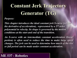
1. Constant Jerk Trajectory Generator(TG) Purpose: This chapter introduces the ideal constant jerk S-curve (jerk is the derivative of acceleration), represented by a 2nd order polynomial in velocity. Its shape is governed by the motion conditions at the start and end of the transition. An S-curve with an intermediate constant acceleration (linear portion) is often used to reduce the time to make large speed changes. The jerk can be used to determine how much of the rise or fall period can be made under constant acceleration.

2. In particular, you will • Determine why S-curves are necessary • Review the ideal S-curve. • Consider constant acceleration jerk transitions. • Consider the speed transition when the velocity change is too small to reach the desired accel (or decel) value. • Consider the trajectory generator in the context of joint moves or curvilinear moves.

3. Why S-curves? 2 v 3 The trapezoidal profile to the right was the trajectory generator of choice for many years, but is now being replaced by S-curve profiles. Why? Area under curve is move distance t 1 4 Reviewing the trapezoidal trajectory profile in speed v, we examine points 1, 2, 3, and 4. Each of these points has a discontinuity in acceleration. This discontinuity causes a very large jerk, which impacts the machine dynamics, also stressing the machine’s mechanical components. An S-curve is a way to impose a limited jerk on the speed transitions, thus smoothing out the robot’s (or machine tool) motion.

4. Ideal S-curve v j as jm 1 vs ar T/2 T 1 t vo Convex Concave T/2 t = T t

5. Ideal S-curve equations The form assumed for the S-curve velocity profile is v(t) = co + c1t + c2 t2 (5.1) giving the acceleration and constant jerk equations: a(t) = c1 + 2 c2 t (5.2) j(t) = 2 c2 (5.3) The rise motion can be divided into 2 periods - a concave period followed by a convex period.

6. v as 1 vs ar 1 vo Convex Concave T/2 t = T t Concave period The concave conditions are v(0) = vo a(0) = 0 a(T/2) = as j(0) = jm where jm is the jerk set for the profile (near the maximum allowed for the robot), and as is the maximum acceleration encountered at the S-curve inflection point.

7. Concave period Applying the initial and final conditions, we get the equations for s (position), v, and a along the concave portion of the S-curve: s(t) = vo t + jm t3/6 (5.7) v(t) = vo + jm t2/2 (5.8) a(t) = jm t (5.9) Note: It is assumed that s is 0 at the beginning of the S-move. Thus, s represents a position delta.

8. Ideal S-curve observations • If we let Dv = vs - vo and define ar = Dv/T to be the acceleration of a constant acceleration ramp from vo to vs, then we note that as is twice ar. It is also true that T = 2Dv/as. • The trapezoidal profile can be used to predict the time and distance required to transition the accel and decel periods of the ideal S-curve. This exercise is commonly called motion or path planning.

9. v as 1 vs ar 1 vo Convex Concave T/2 t = T t Convex period This period applies for T/2 £ t £ T. Letting time be zero measured from the beginning of the convex period (0 £ t £ T/2), the pertinent motion conditions are: v(0) = vh = (vs + vo)/2 a(0) = as a(T/2) = 0 j(0) = -jm where -jm is the jerk set for the profile, and as is the maximum acceleration encountered at the S-curve inflection point.

10. Convex period Applying the initial and final conditions, we get the equations for s (position), v, and a along the convex portion of the S-curve: s(t) = vh t + as t2/2 - jm t3/6 (5.11) v(t) = vh + as t - jm t2/2 (5.12) a(t) = as - jm t (5.13) Note: It is assumed that s is 0 at the beginning of the S-move. Thus, s represents a position delta.

11. Distance traversed Adding in the distance at the halfway point gives the total distance traversed in the S-curve, including both concave and convex sections: S = (vs2 - vo2)/as

12. Max jerk transitions An ideal S-curve cannot transition smoothly between any speed change using a specified max jerk value! Why?

13. Max jerk transitions Given a jerk jm, a starting speed vo, and the ending speed vs, we can determine v1 and v2, where these are the velocities that end the concave transition and begin the convex transition at max accel as for the ideal S-curve transition: v1 = vo + as2/(2jm) v2 = vs- as2/(2 jm) By setting v1 = v2, we can also determine the max jerk for a given as and Dv = vs - vo: jm = as2 /Dv

14. Speed transitions If v1 > v2 (overlap), we can determine an intermediate transition point using speed and acceleration continuity. Note that the velocity and acceleration for the previous concave curve and the new convex curve must be equal at Tt where the velocity is vt. We cannot reach the maximum acceleration as by applying maximum jerk transitions. Nevertheless, there exists a point where the concave profile will be tangent to the convex profile. This point will lie between vo and vs. At this point the acceleration and speed of both profiles are the same, although there will be a sign change in jerk.

15. Speed transitions The pertinent equations are: vo + ao Tt + jm Tt 2/2 = vs- jm (T - Tt)2/2 (5.20) ao + jm Tt = jm (T - Tt) (5.21) Solving these we get: T = [-ao + sqrt( 2 ao2 + 4 Dv jm) ]/ jm (5.22) Tt = (jm T - ao)/(2 jm) (5.23) where Dv = (vs - vo).

16. v j as jm 1 vs ar T-t1 t = T 1 t1 t vo t1 t t = T S-Curve profile with linear period S-curve with linear period If v1 < v2, then we must insert a linear (constant acceleration) period. The desired maximum S accel (as) is known, as is the maximum jerk (jm).

17. S-curve with linear period Motion conditions: Phase 1 - Concave       Phase 2 – Linear Phase 3 - Convex 0 £ t £ t10 £ t £ T -2t1 0 £ t £t1_________________________________________________________________________________________________________________ v(0) = vo a(0) = 0 a(t1) = as j(0) = jm v(t1) = v1 v(0) = v1 a(0) = as a(T-2t1) = as v(T-2t1) = v2 v(0) = v2 a(0) = as v(t1) = vs a(t1) = 0 j(0) = - jm

18. S-curve with linear period Phase 1 – Concave motion conditions: s(t) = vo t + jm t3/6 (5.25) v(t) = vo + jm t2/2 (5.26) a(t) = jm t (5.27)

19. S-curve with linear period Phase 2 – Linear motion conditions: s(t) = v1 t + as t2/2 (5.30) v(t) = v1 + as t (5.31)

20. S-curve with linear period Phase 3 – Convex motion conditions: s(t) = v2 t + as t2/2 - jm t3/6 (5.35) v(t) = v2 + as t - jm t2/2 (5.36) a(t) = as - jm t (5.37)

21. S-curve context How is the S-curve applied in the real world? Robots and machine tools are commanded to move in either joint space or Cartesian space. In joint space the slowest joint becomes the controlling move. Its set speed and joint distance is used for the trajectory motion planning. Desired acceleration and jerk values are applied for this joint to specify the S-curve profiles. In Cartesian space either the path length or tool orientation change dominates the motion. The associated speeds , accelerations, and jerk values specify the S-curve profiles. The trajectory generator processes length or orientation change, whichever is dominant. The other change is proportioned.

22. TG summary • S-curve is used to smooth speed transitions by eliminating points of extremely high jerk. • S-curve is limited by jerk and acceleration settings, and also by desired speed change. • The equations that govern the decel period of the TG are similar to the accel period, but use a negative acceleration setting. • The S-curve profiles can be applied to joint moves or to Cartesian moves.