Download

1 / 30
300 likes | 428 Views
Image Features - I. Hao Jiang Computer Science Department Sept. 22, 2009. Outline. Summary of convolution and linear systems Image features Edges Corners Programming Corner Detection. Properties of Convolution. 1. Commutative: f * g = g * f 2. Associative

E N D
Image Features - I Hao Jiang Computer Science Department Sept. 22, 2009
Outline • Summary of convolution and linear systems • Image features • Edges • Corners • Programming Corner Detection
Properties of Convolution 1. Commutative: f * g = g * f 2. Associative (f * g) * h = f *(g * h) 3. Superposition (f + g) * h = f * h + g * h N M full (N+M-1)x(N+M-1)
Linear System f h g = f * h Linear: a f1+ b f2 => a g1 + b g2 where the response of f1 is g1 and the response of f2 is g2 Shift invariant: if f => g, then f(n-m) => g(n-m)
Composite Linear System f h1 h2 h1 + h2 f h1 h2 h1*h2
Nonlinear Filtering • Neighborhood filtering can be nonlinear • Median Filtering • 1 1 • 1 2 1 • 1 1 1 Mask [1 1 1 ] • 1 1 • 1 1 1 • 1 1 1
Median Filtering in Denoising Original Image Add 10% pepper noise
Median Filtering for Denoising Median filter with 3x3 square structure element
Median Filtering for Denoising Median filter with 5x5 square structure element
Compared with Gaussian Filtering Kernel size 5x5 and sigma 3 Kernel size 11x11 and sigma 5
Image Local Structures Step Ridge Valley Peak Corner Junction
Image Local Structures Line Structures: “Edge” Step Ridge Valley Point Structures: “Corners” Peak Corner Junction
An Example edge Region corners
Edge Detection in Matlab >> im = imread('flower.jpg'); >> im = im2double(im); >> im = rgb2gray(im); >> ed = edge(im, 'canny', 0.15);
How to Find an Edge? A 1D edge
f(x) f’(x) f’’(x)
Extend to 2D b There is a direction in which image f(x,y) increases the fastest. The direction is called the gradient direction. Gradient [df/dx df/dy] Magnitude: sqrt(fx^2 + fy^2) Direction: atan2(fy, fx) a
Finite Difference • Approximating derivatives using finite difference. • Finite difference and convolution
Noise Reduction 0.01 noise 0.03 noise
Gaussian Filtering in Edge Detection image h * (g * f) = (h * g) * f Difference of Gaussian Kernel Difference Kernel Gaussian Kernel
Edge Detection in Images • Gaussian smoothed filtering in x and y directions: Ix, Iy • Non-maximum suppression for |Ix|+|Iy| • Edge Tracing – double thresholding.
Edge Detection Using Matlab • Canny edge detector: edge(image, ‘canny’, threshold) • Sobel edge detector: edge(image, ‘sobel’, threshold) • Prewitt edge detector: edge(image, ‘prewitt’, threshold)
Berkeley Segmentation DataSet [BSDS] D. Martin, C. Fowlkes, D. Tal, J. Malik. "A Database of Human Segmented Natural Images and its Application to Evaluating Segmentation Algorithms and Measuring Ecological Statistics”, ICCV, 2001
Corner Detection • Corner is a point feature that has large changing rate in all directions. Peak Step Line Flat region
Find a Corner Compute matrix H = Ix2 Ixy Ixy Iy2 = in each window. If the ratio (Ix2 * Iy2 – Ixy ^2 ) ------------------------ > T (Ix2 + Iy2 + eps) We have a corner