Download
1 / 37
370 likes | 476 Views
-X. -Y. Y. X. the strange geometries of computer science. James R. Lee. University of Washington. TexPoint fonts used in EMF. Read the TexPoint manual before you delete this box.: A A A A A. part I: intrinsic dimensionality and nearest-neighbor search [with Krauthgamer].

E N D
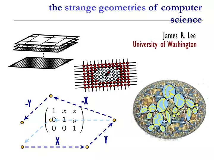
-X -Y Y X the strange geometries of computer science James R. Lee University of Washington TexPoint fonts used in EMF. Read the TexPoint manual before you delete this box.: AAAAA
part I: intrinsic dimensionality and nearest-neighbor search [with Krauthgamer] three geometries part II: the heisenberg geometry and sparse cuts in graphs [with A. Naor] part III: negative curvature and traveling salesmen [with Krauthgamer]
part I: intrinsic dimensionality and nearest-neighbor search [with Krauthgamer] three geometries part II: the heisenberg geometry and sparse cuts in graphs [with Naor] part III: negative curvature and traveling salesmen [with Krauthgamer]
The problem: We are given some set S of n points lying in a huge (possibly infinite) metric space (M, d). nearest-neighbor search Want to preprocess S so that given a query q 2 M, we can efficiently locate the nearest point to q among those in S. (Other concerns: Insertion/deletion of points from S.) Basic question: For general metric spaces, how efficient can a search algorithm be? For which spaces do efficient algorithms exist? (M, d) S q
Problem: (1+)-NNS approximate NNS • Want to preprocess S so that given a query q 2 M, we can • efficiently locate a point a 2 S such that d(q,a) · (1+) d(q,S) • Application domain: General metric spaces • Most previous work focused on the special case where M = Rd • is equipped with some Lp norm. Unnatural for many applications. • We focus on general spaces and access the query using the distance • function as an oracle, e.g. d(q, ¢). (Ad-hoc networks, manifold data, databases, biological data, …)
Suppose that (S, d) is a uniform metric: d(x,y) = 18 x,y 2 S. a hard example (lack of information) Same example works even if S is only a “near-uniform” metric. S 1 1 Need some way of deciding tractability. 1 Have to do exhaustive search.
Definition: A metric space (X,d) is doubling if there exists a constant • such that every ball in X can be covered by balls of half the radius. bounding the geometry r = 5 If (X) is the minimum over all such , we define dim(X) = log2(X) [GKL03] (“scaled down” notion a la Assouad’83)
structural properties doubling dimension - dim(Rd) ¼ d (under any norm) - X µ Y ) dim(X) · dim(Y) - dim(X) · log|X| algorithmic properties There exists a (1+)-NNS data structure using: SPACE: O(n) QUERY TIME:4dim(X) O(log n) + O(2/)dim(X) UPDATE TIME: O(log n) [Cole-Gottlieb 06, HarPeled-Mendel 05, KLa 04, KLb 04]
nets and dimension (X,d) A subset N µ X is called an -net if • d(x,y) ¸8 x y 2 N • X µ[y 2 N Ball(y,) x Easy lemma: If N is an -net in X, then |N Å Ball(x,R)| · (2R/)dim(X) (bounds the size of “near-uniform” sets in X)
basic algorithm The basic data structure is a sequence of progressively finer -nets for = 2k, 2k-1, … To make one step, we only need to decide between 4dim(X) points. Every step reduces distance to the query by a factor of 2.
(M, d) S q efficient NNS data structure $dim(S) small if we want to answer any possible query from the ambient space M. related results - Implementation called “Cover Trees” by BKL used in isomap and beats popular hierarchical search approaches (e.g. ball trees) - Used in many other contexts (e.g. internet routing, peer-to-peer networks, approximation algorithms...)
part I: intrinsic dimensionality and nearest-neighbor search [with Krauthgamer] heisenberg geometry part II: the heisenberg geometry and sparse cuts in graphs [with Naor] part III: negative curvature and traveling salesmen [with Krauthgamer]
S E(S, S) Input: A graph G=(V,E). sparsest cut: edge expansion For a cut (S,S) let E(S,S) denote the edges crossing the cut. The sparsity of S is the value The SPARSEST CUT problem is to find the cut which minimizes (S). This problem is NP-hard, so we try to find approximatelyoptimal cuts. (approximation algorithms)
semi-definite relaxation Leighton and Rao gave an O(log n) approximation based on Linear Programming/ Multi-commodity flows (1988). To do better, we look at semi-definite programs. integer formulation: SDP formulation: valid 0/1 constraint:
2nd eigenvalue of the Laplacian of the graph G (spectral approach) semi-definite relaxation combines power of spectral and flow-based approaches add the valid “triangle inequality” constraints: for all u,v,w 2 V final SDP:
squared L2 distance: negative type metrics These constraints imply that the function d(u,v) = (xu-xv)2 is a metric (i.e. it satisfies the triangle inequality). These are called negative type or squared-L2 metrics. Impose strong geometric constraints on the solution: xu · 90o xv xw
upper bounds SDP analysis results uniform version: [Arora-Rao-Vazirani 04] non-uniform version: [Arora-L-Naor 05] lower bounds [Krauthgamer-Rabani 06] non-uniform version: [Devanur-Khot-Saket-Vishnoi 06] uniform version: Lower bounds (starting with Khot-Vishnoi) were hard because vectors satisfying these constraints are in short supply:
Consider the group of upper triangular matrices with integer entries (under matrix multiplication) the heisenberg group Let G(H3) be the Cayley graph of H3(Z) with generators: X -X Y -Y BUT…
-X -Y the heisenberg group Y X X -X Y -Y BUT…
-X -Y the heisenberg group Y X X -X Y -Y ALL MOVEMENT IS “INFINITESIMALLY” HORIZONTAL
the heisenberg group X -X Y -Y The space G(H3)is translation invariantand homogeneous but not isotropic. Using H3-analogues of Fourier analysis in the classical setting of Rd, we are able to show (with A. Naor) that the shortest-path metric on G(H3) is of negative type. We conjectured that G(H3) does not embed in L1, and this was proved recently by J. Cheeger and B. Kleiner
Cheeger and Kleiner (wrong attribution and informal version): local rigidity in H3 If S µH3 is a set with “small perimeter”, then locallyS looks like a vertical hyperplane in R3. X Y
part I: intrinsic dimensionality and nearest-neighbor search [with Krauthgamer] negatively curved spaces part II: the heisenberg geometry and sparse cuts in graphs [with Naor] part III: negative curvature and traveling salesmen [with Krauthgamer]
why negative curvature? - Extensive theory of computational geometry in Rd. What about other classical geometries? (e.g. hyperbolic) Eppstein: Is there an analogue of Arora’s TSP alg for H2? - Class of “low-dimensional” spaces with exponential volume growth, in contrast with other notions of “intrinsic” dimension (e.g. doubling spaces) - Natural family of spaces that seem to arise in applied settings (e.g. networking, vision, databases) Modeling internet topology [ST’04], genomic data [BW’05] Similarity between 2-D objects (non-positive curvature) [SM’04]
x (x|y) r y Gromov -hyperbolicity what’s negative curvature? For a metric space (X,d) with fixed basedpoint r 2 X, we define the Gromov product (x|y) = [d(x,r) + d(y,r) – d(x,y)]/2. [For a tree with root r, (x|y) = d(r, lca(x,y)).] (X,d) is said to be -hyperbolic if, for every x,y,z 2 X, we have (x|y) ¸ min{(x|z), (y|z)} - [A tree is 0-hyperbolic.] Aside: How do we represent our manifold…?
x y z Thin triangles what’s negative curvature? (geodesic spaces) A geodesic space is -hyperbolic (for some ) if and only if every geodesic triangle is -thin (for some ). geodesics [x,y], [y,z], [x,z] -thin: every point of [x,y] is within of [y,z][ [x,z] (and similarly for [y,z] and [x,z])
Exponential divergence of geodesics what’s negative curvature? (geodesic spaces) A geodesic space is -hyperbolic (for some ) if and only every pair of geodesics “diverges” at an exponential rate. t=t1 t=t0 x threshold length(P) ¸ exp(t1-t0) P y z
Make various assumptions on the space locally - locally doubling (every small ball has poly volume growth) - locally Euclidean (every small ball embeds in Rk for some k) and globally - geodesic (every pair of points connected by a path) - -hyperbolic for some ¸ 0 e.g. bounded degree hyperbolic graphs, simply connected manifolds with neg. sectional curvature (e.g. Hk), word hyperbolic groups results Most of our algorithms are intrinsic in the sense that they only need access to a distance function d (not a particular representation of the points or geodesics, etc.)
what we can say… (with Krauthgamer) - Linear-sized (1+)-spanners, compact routing schemes, etc. • Nearest neighbor search data structure with • O(log n) query time, O(n2) space • PTAS (approx. scheme) for TSP, and other Arora-type problems
random tesellations: how’s the view from infinity? boundary at infinity 1H2 equivalence classes of geodesic rays emenating from the origin - Two rays are equivalent if they stay within bounded distance forever - Natural metric structure on 1H2 Bonk and Schramm: If the space is locally nice (e.g. locally Euclidean or bounded degree graph), then 1H2 has small doubling dimension.
Use hierarchical random partitions of 1X to construct random tessellations of X. random tessellations: how’s the view from infinity? Now let’s see how to use this for finding near-optimal TSP tours…
log n n/2 MST 1 OPT Tree doubling ain’t gonna cut it… the approximate TSP algorithm differ by 2-o(1) factor
metric spaces tree of metric spaces: family of metric spaces glued together in a tree-like fashion the approximate TSP algorithm
the approximate TSP algorithm THEOREM. For every >0, and d¸1, there exists a number D(,d) such that every finite subset X µHd admits a (1+)-embedding into a distribution over dominating trees of metric spaces where the constituent spaces admit each admit an embedding into Rd with distortion D(,d).
the approximate TSP algorithm THEOREM. For every >0, and d¸1, there exists a number D(,d) such that every finite subset X µHd admits a (1+)-embedding into a distribution over dominating trees of metric spaces where the constituent spaces admit each admit an embedding into Rd with distortion D(,d). - In other words, we have a random map f : X ! T({Xi}) where T({Xi}) is a random tree of metric spaces with induced metric dT whose constituent spaces are the {Xi}. - For every x,y 2 X we have dT(f(x),f(y)) ¸ d(x,y). - For every x,y 2 X we have
the approximate TSP algorithm ALGORITHM. - Sample a random map f : X ! T({X1, X2, …, Xm}) • For each k=1,2,…,m, use Arora’ to compute a near- • optimal salesman tour for every distorted Euclidean piece Xk. • Output the induced tour on X. X
part I: intrinsic dimensionality and nearest-neighbor search [with Krauthgamer] conclusion part II: the heisenberg geometry and sparse cuts in graphs [with Naor] part III: negative curvature and traveling salesmen [with Krauthgamer]