Download
1 / 35
370 likes | 452 Views
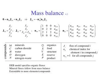
Mass balance 4.3. minerals carbon dioxide water dioxygen nitrogen-waste. organics food structure reserve product. flux of compound i chemical index for element i in compound j for all compounds j. compounds. DEB model specifies organic fluxes

E N D
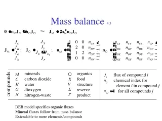
Mass balance 4.3 minerals carbon dioxide water dioxygen nitrogen-waste organics food structure reserve product flux of compound i chemical index for element i in compound j for all compounds j compounds DEB model specifies organic fluxes Mineral fluxes follow from mass balance Extendable to more elements/compounds
Mass-energy coupling 4.3 Organic fluxes are linear combinations of 3 energy fluxes organics food structure reserve product assimilation dissipation growth chemical potential of E yield of compound i on j coupler of compound i to power j for faeces: compounds powers Decomposition of mineral fluxes into contributions from 3 basic energy fluxes:
Energy balance 4.9.1 Dissipating heat can be decomposed into contributions from 3 basic energy fluxes chemical potentials (energy-mass couplers) mass-energy couplers fluxes of compounds 3 basic energy fluxes (powers) chemical indices minerals organics
Method of indirect calorimetry 4.9.2 Empirical origin (multiple regression): Lavoisier 1780 Heat production = wC CO2-production + wO O2-consumption + wN N-waste production DEB-explanation: Mass and heat fluxes = wA assimilation + wD dissipation + wG growth Applies to CO2, O2, N-waste, heat, food, faeces, … For V1-morphs: dissipation maintenance
Mass fluxes 4.1 allocation to reproduction flux use of reserve not balanced by feeding in embryo flux notice small dent due to transition maturation reproduction At abundant food: growth ceases at l = 1
Methanotrophy 4.3.1 Yield coefficients Y and chemical indices n depend on (variable) specific growth rate r For reserve density mE = ME/MV (ratio of amounts of reserve and structure), the macroscopic transformation can be decomposed into 5 microscopic ones with fixed coefficients C: carbon dioxide N: ammonia O: dioxygen V: structure X: methane E: reserve H: water process symbol rate Yield coefficientsT Chemical indices
Methanotrophy 4.3.1 C E X/O N flux ratio, mol.mol-1 spec flux, mol.mol-1.h-1 N/O C/O X O spec growth rate, h-1 spec growth rate, h-1 X: methane C: carbon dioxide O: dioxygen N: ammonia E: reserve jEAm = 1.2 mol.mol-1.h-1 yEX = 0.8 yVE = 0.8 kM = 0.01 h-1 kE = 2 h-1 chemical indices nHE = 1.8 nOE = 0.3 nNE = 0.3 nHV = 1.8 nOV = 0.3 nNV = 0.3 Kooijman, Andersen & Kooi 2004. Ecology, to appear
Biomass composition 4.3.4 Data Esener et al 1982, 1983; Kleibsiella on glycerol at 35°C nHW Entropy J/C-mol.K Glycerol 69.7 Reserve 74.9 Structure 52.0 Sousa et al 2004 Interface, subm Relative abundance nOW O2 nNW Weight yield, mol.mol-1 Spec prod, mol.mol-1.h-1 Spec growth rate, h-1 CO2 Spec growth rate kE 2.11 h-1 kM 0.021 h-1 yEV 1.135 yXE 1.490 rm 1.05 h-1 g = 1 nHE 1.66 nOE 0.422 nNE 0.312 nHV 1.64 nOV 0.379 nNV 0.189 Spec growth rate, h-1
Product Formation 4.7 According to Dynamic Energy Budget theory: Product formation rate = wA. Assimilation rate + wM. Maintenance rate + wG . Growth rate For pyruvate: wG<0 ethanol pyruvate, mg/l pyruvate glycerol, ethanol, g/l glycerol throughput rate, h-1 Glucose-limited growth of Saccharomyces Data from Schatzmann, 1975
Reserve Capacity & Growth low turnover rate: large reserve capacity high turnover rate: small reserve capacity
Multivariate extensions 5 animal heterotroph phototroph plant symbiosis
Photosynthesis 5.1.3 2 H2O + 4 h O2 + 4 H+ + 4 e- CO2 + 4 H+ + 4 e- CH2O + H2O CO2 + H2O + light CH2O + O2
Simultaneous nutrient limitation 5.2.3 Specific growth rate of Pavlova lutheri as function of intracellular phosphorus and vitamine B12 at 20 ºC Data from Droop 1974 Note the absence of high contents for both compounds due to damming up of reserves, and low contents in structure (at zero growth)
Reserve interactions 5.2.4 Data from Droop 1974 on Pavlova lutheri B12-cont., 10-21.mol.cell-1 P-content, fmol.cell-1 P-conc, μM B12-conc, pM Spec growth rate, d-1 Spec growth rate, d-1 Spec growth rate, d-1
Steps in food 7.1.2 Growth of Daphnia magna at 2 constant food levels 0 d 7 d 14 d 21 d • Only curves at • 0 d are fitted • Notice • slow response • gut content in • down steps length, mm Steps up length, mm Steps down time, d time, d time, d time, d
Growth on reserve 7.1.3 Conc. potassium, mM Optical Density at 540 nm time, h Potassium limited growth of E. coli at 30 °C Data Mulder 1988; DEB model fitted OD increases by factor 4 during nutrient starvation internal reserve fuels 9 hours of growth
Growth on reserve 7.1.3 Growth in starved Mytilus edulis at 21.8 °C Data Strömgren & Cary 1984; DEB model fitted internal reserve fuels 5 days of growth growth rate, mm.d-1 time, d
Protein synthesis 7.5 scaled elongation rate RNA/dry weight, μg.μg-1 Data from Bremer & Dennis 1987 Data from Koch 1970 spec growth rate, h-1 scaled spec growth rate RNA = wRV MV + wRE ME dry weight = wdV MV + wdE ME
Scales of life 8.0 Life span 10log a Volume 10log m3 earth life on earth whale whale bacterium ATP bacterium water molecule
Invariance property 8.1 The parameters of two individuals can differ in a very special way such that both individuals behave identically at constant food density if they start with the same values for the state variables (reserve, structure, damage) At varying food density, two individuals only behave identically if all their parameters are equal
Inter-species body size scaling 8.2 • parameter values tend to co-vary across species • parameters are either intensive or extensive • ratios of extensive parameters are intensive • maximum body length is • allocation fraction to growth + maint. (intensive) • volume-specific maintenance power (intensive) • surface area-specific assimilation power (extensive) • conclusion : (so are all extensive parameters) • write physiological property as function of parameters • (including maximum body weight) • evaluate this property as function of max body weight Kooijman 1986 Energy budgets can explain body size scaling relations J. Theor. Biol.121: 269-282
Primary scaling relationships assimilation {JEAm} max surface-specific assim rate Lm feeding {b} surface- specific searching rate digestion yEX yield of reserve on food growth yVEyield of structure on reserve mobilization v energy conductance heating,osmosis {JET} surface-specific somatic maint. costs turnover,activity [JEM] volume-specific somatic maint. costs regulation,defence kJ maturity maintenance rate coefficient allocation partitioning fraction egg formation R reproduction efficiency life cycle [MHb] volume-specific maturity at birth life cycle [MHp] volume-specific maturity at puberty aging ha aging acceleration Kooijman 1986 J. Theor. Biol. 121: 269-282 maximum length Lm = {JEAm} / [JEM]
Initial reserve of an egg • Follows from: • maturity at birth equals a given value • reserve density at birth equals that of mother • State variables: • Parameters: • Problem: Given parameter values, find Theory in Kooy2008
Effects of nutrition scaled length at birth scaled age at birth scaled res density at birth scaled res density at birth scaled initial reserve scaled res density at birth
Reduction of initial reserve scaled maturity 1 scaled reserve 0.8 0.5 scaled age scaled age scaled struct volume scaled age
Scaling relationships log scaled initial reserve log scaled age at birth log zoom factor, z log zoom factor, z approximate slope at large zoom factor log scaled length at birth log zoom factor, z
Lp, cm L, cm Length at puberty 8.2.1 Clupoid fishes Sardinella + Engraulis * Centengraulis Stolephorus Clupea • Brevoortia ° Sprattus Sardinops Sardina Data from Blaxter & Hunter 1982 Length at first reproduction Lp ultimate lengthL
Body weight 8.2.2 Body weight has contribution from structure and reserve If reserves allocated to reproduction hardly contribute: intra-spec body weight inter-spec body weight intra-spec structural volume Inter-spec structural volume reserve energy compound length-parameter specific density for structure molecular weight for reserve chemical potential of reserve maximum reserve energy density
Feeding rate 8.2.2 slope = 1 Filtration rate, l/h Mytilus edulis Data: Winter 1973 poikilothermic tetrapods Data: Farlow 1976 Length, cm Inter-species: JXm V Intra-species: JXm V2/3
Scaling of metabolic rate 8.2.2 Respiration: contributions from growth and maintenance Weight: contributions from structure and reserve Structure ; = length; endotherms
Metabolic rate 8.2.2 slope = 1 Log metabolic rate, w O2 consumption, l/h 2 curves fitted: endotherms 0.0226 L2 + 0.0185 L3 0.0516 L2.44 ectotherms slope = 2/3 unicellulars Log weight, g Length, cm Intra-species Inter-species (Daphnia pulex)
Von Bertalanffy growth rate 8.2.2 25 °C TA = 7 kK 10log von Bert growth rate, a-1 10log ultimate length, mm 10log ultimate length, mm At 25 °C : maint rate coeff kM = 400 a-1 energy conductance v = 0.3 m a-1 ↑ ↑ 0