Download
1 / 24
240 likes | 269 Views
Learn how LiDAR technology was used to map sinkholes and potential groundwater recharge zones in Jefferson County, WV, as part of a USGS study. See the process of data acquisition, processing, and field verification to identify sinkholes accurately. Discover other applications of LiDAR beyond sinkhole mapping.

E N D
Using LiDAR to map sinkholes in Jefferson County, West Virginia John Young, USGS Leetown Science Center Kearneysville, WV
“I read the news today, oh boyFour thousand holes in Blackburn, LancashireAnd though the holes were rather smallThey had to count them all…” A Day in the Life The Beatles
Project Objectives * Part of a USGS study of water availability and threats to water supply of the Leetown Science Center (Kozar et al. 2007) • Acquire LiDAR data to allow for modeling of fine scale surface features • Generate fine-scale digital elevation models from LiDAR data • Use topographic analysis, aerial photography, and statistical analysis to map sink holes and potential groundwater recharge zones from fine-scale surface models
What is LiDAR? • LiDAR = Light Detection And Ranging (aka “airborne laser scanning”) • Laser pulses sent from aircraft in dense scanning pattern (0.5-2 meters apart) • Return of laser pulse recorded at aircraft • Time to return, speed of light, and altitude of plane used to compute surface height (z) of each pulse with high accuracy • Ground position of each laser pulse computed using differential GPS (x,y)
What is LiDAR? Image courtesy: www.chez.com
LiDAR returns (overlaid on aerial photograph) LiDAR returns: First (top of canopy, roofs), Last (ground surface)
Data Acquisition • Acquired LiDAR data by partnering with USDA-NRCS • Conducted accuracy assessment of LiDAR data acquisition in exchange for access to data • LiDAR flight of Jefferson County WV, by Sanborn, Inc. in April 2005 (leaf off) • LiDAR data delivered as first return, last return, and “bare earth” (vegetation and buildings removed) • 81 tiles (1/16th quad) • < 1.0 meter point spacing
USGS QA/QC Campaign: • 38 stations established throughout county in variety of land surface types • Survey-grade GPS used to collect surface height data • GPS surface heights compared to mean LiDAR return height within 2 meters of GPS points • All but 1 checkpoint were within ± 0.15 meter RMSE (< FEMA spec)
Problem: Find method to locate surface sinks, even under forest canopy Color Aerial Photo, 0.6 meter pixel resolution, 2003
Data: LiDAR, acquired Spring 2005, delivered Fall 2005 Raw (last return) data gridded to 2m surface
Progressive Curvature Filtering • Evans and Hudak (2007) proposed a method for processing LiDAR data to find ground surface in forests of the interior western U.S. • Method uses an adaptive, iterative filter that considers scale of variation • Fits “thin-plate splines with tension” at multiple scales to examine local curvature and determine which points to filter out • Effective at removing vegetation
Data processing: Progressive Curvature Filter (Evans and Hudak, 2006) PCF filtered data gridded to 2m surface Raw (unflitered) last return data, gridded to 2m
Data processing: a modification of McNab’s (1989) “Terrain Shape Index” TSI = DEMgrid – focalmean(DEMgrid, annulus, 1, 5) Focal cell higher than surrounding cells = convex Focal cell lower than surrounding cells = concave * Graphic after F. Biasi (TNC)
Data processing: Landform analysis Landform shape in 10 m window, red = concave, blue = convex
Data processing: Landform assessment Find compact bowl features, possible sinkholes
Field Verification Sinkhole = yes!
Field validation results94 sites mapped, 55 visited on ground Sink (throat) found: 16.4% Probable sink (no throat): 43.6% Depression: 25.5% Not a sink: 14.5%
Other applications of LiDAR • Site analysis • Geologic structure • Fault line tracing • Hydrology / floodplain assessments • Vegetation height/structure • Slope analysis • ??
Conclusions • PCF filtered LiDAR data provided a high resolution “bare earth” elevation surface • Converting elevation values into a landform shape index was effective at highlighting depression features • Caveat: Depression ≠ sinkhole (but it’s a good place to start looking!) For additional info, contact John Young (jyoung@usgs.gov)
Acknowledgements • Jared Beard, USDA-NRCS soil scientist, Moorefield, WV (collaborator) • John Jones, USGS Geography division, Reston, VA (collaborator) • Bob Glover, USGS Geography division, Reston, VA (GPS survey) • Jeffrey Evans, USFS, Moscow, Idaho (filtering algorithms) • Kenny Legleiter, (formerly of) USDA-NRCS, Ft. Worth, TX (LiDAR flight contracting) • Data acquired by Sanborn, Inc. under contract to USACE/USDA-NRCS