Prerequisites for a Scientific Visualization course
400 likes | 427 Views
This course covers the fundamentals of scientific visualization, including techniques for taking images, arranging scenes, and using graphics libraries like OpenGL. Topics also include geometric transformations and various graphics algorithms.

Prerequisites for a Scientific Visualization course
E N D
Presentation Transcript
Prerequisites for a Scientific Visualization course Michel O. R. Eboueya Computer Science, Maths & Applications Department Pôle Sciences et Technologies Université de La Rochelle
Outline Know how to take an image References and Example of a Computer Graphics Course Survival concepts Line & Circle generation Clipping (2 methods) Curves and surfaces (just Bezier) Ray Casting (well known) To Scientific Visualization
Know how to take an image Arrange the scene model MODEL Point the camera to the direction of the scene, VIEW Tune the camera lenses ( zoom. . .) PROJECTION Size of the picture and clic VIEWPORT Using a Graphics Library…OpenGL
Know how to take an image Arrange the scene model MODEL Point the camera to the direction of the scene, VIEW Tune the camera lenses ( zoom. . .) PROJECTION Size of the picture and clic VIEWPORT Using a Graphics Library…OpenGL
Outline Know how to take an image References and Example of a Computer Graphics Course Survival concepts Line & Circle generation Clipping (2 methods) Curves and surfaces (just Bezier) Ray Casting (well known) To Scientific Visualization
Bibliographie 1) J. D. Foley & A.Van Dam Fundamentals of Interactive Computer Graphics Addison-Wesley Publishing Company 2) Interactive Computer Graphics . A top down approach with OpenGL. Adward Angel Addison Wesley 3) Computer Graphics Mathematical first steps . P.A. Egerton et W.S Hall Prentice Hall Europe All topics complemented with practical implementations using Open GL (wintel or linux) to encourage a "hands-on" or "learning-by-doing" attitude.
Exemple de cours complet 01 - Linear Algebra a. Matrix b. Polynomials c. Linear Transformations 02 - Computational Geometry a. geometric searching b. Convex Hulls c. Proximity d. Intersections e. The Geometry of Rectangles
Exemple de cours complet 03 - Graphics Hardware a. Display Technologies b. Raster-Scan Display Systems c. The Video Controller 04 - 2D and 3D Transformations a. Translations b. Rotations c. Scaling d. Reflections e. Composition of Transformations
Exemple de cours complet 05 - Viewing in 2D and 3D a. Homogeneous Coordinates b. Parallel Projections c. Perspective Projections d. View Volume e. Clipping f. Viewport Mapping and Window Mapping g. Viewing Transformations 06 - Curves and Surfaces a. Polygon Meshes b. Parametric Cubic Curves c. Parametric Bicubic Surfaces d. Quadric Surfaces
Exemple de cours complet 07 - Solid Modelling a. Solid Representation b. Regularized Boolean Set Operations c. Primitive Instancing d. Sweep Representations e. Boundary Representations f. Constructive Solid Geometry g. User Interfaces for Solid Modelling 08 - Achromatic and Colored Light a. Color and Light in Computer Graphics b. Achromatic Light c. Chromatic Color d. Color Models for Raster Graphics e. Reproducing Color in Computer Graphics
Exemple de cours complet 09 - Aliasing and Antialiasing Techniques a. Sampling Theory b. Point Sampling c. Area Sampling d. Stochastic Sampling e. Filtering f. Image Reconstruction
Exemple de cours complet 10 - Visible-Surface Determination a. Functions of Two Variables b. Coherence c. Extents and Bounding Volume d. Spatial Partitioning f. Hierarchy g. Algorithms for Visible-Line Determination h. The Z-Buffer Algorithm i. List-Priority Algorithms j. Scan-Line Algorithms k. Area-Subdivision Algorithms l. Algorithms for Octrees m. Algorithms for Curved Surfaces
Exemple de cours complet 11 - Illumination and Shading a. Illumination Models b. Shading Models c. Transparency Models d. Interobject Reflections e. Physically Based Illumination Models f. Light Sources g. Local Illumination Algorithms h. Global Illumination Algorithms i. Radiosity Methods
Exemple de cours complet 12 - Texture Techniques a. Texture Mapping b. Bump Mapping c. Displacement Mapping 13 - Ray Tracing a. Theory b. Visible-Surface Ray Tracing c. Recursive Ray Tracing 14 - Image Manipulation And Storage a. Image Processing b. Geometric Transformation of Images c. Multipass Transformations d. Image Compositing e. Mechanisms for Image Storage f. Special Effects with Images
Exemple de cours complet 15 - Computer-Assisted Animation and Simulation a. Animation Languages b. Methods of Controlling Animation c. Basic Rules of Animation d. Interactive Computer Graphics Animation e. Real-Time Simulation 16 - Advanced Raster Graphics Architecture and Techniques a. Frame-Buffer b. Dynamic Memories c. The Video RAM d. Display-Processor Systems e. Standard Graphics Pipeline f. Introduction to Multiprocessing g. Pipeline Front-End Architectures h.Parallel Front-End Architectures i. Multiprocessor Rasterization Architectures j. Image-Parallel Rasterization k. Object-Parallel Rasterization l. Hybrid-Parallel Rasterization m. Enhanced Display Capabilities n. Advanced Geometric and Raster Algorithms o. Advanced Modelling Techniques
Algorithme de Cohen-Sutherland (3/ 2eme étape de l'algorithme de Cohen-Sutherland : si les codes des 2 extrémités sont tous 2 égaux à 0000, le segment est visible si le résultat d'un ET logique sur les 2 codes est différent de 0000, il est invisible si le résultat d'un ET logique sur les 2 codes est égal à 0000, le segment est candidat au fenêtrage.
Algorithme de Cohen-Sutherland (4/ Puis, calcul des Intersection des segments et fenêtrage pour les segments candidats au fenêtrage. Cas des fenêtres dont les côtés sont parallèles aux axes de coordonnées : les côtés de la fenêtre susceptibles de couper le segment sont ceux vers lesquels les extrémités du segment devraient être ramenées si l'on voulait changer les 1 de leur code en 0. Si b1=1 intersection possible avec y = ymax b2=1 y = ymin b3=1 x = xmax b4=1 x = xmin
Algorithme de Sutherland-Hodgman On considère le côté Pi-1 Pi 1) si Pi et Pi -1 sont tous deux à gauche du côté E, le sommet Pi est placé dans la liste des sommets du polygone fenêtré. 2) si Pi-1 et Pi sont tous deux à droite du côté E, rien n'est placé dans la liste des sommets du polygone fenêtré 3) si Pi-1 est à gauche et Pi à droite du côté E, le point d'intersection I du segment Pi-1 Pi avec le prolongement du côté E est calculé et placé dans la liste des sommets du polygone fenêtré 4) si Pi-1 est à droite et Pi à gauche du côté E, le point d'intersection I du segment Pi-1 Pi avec le prolongement du côté E est calculé. On place I et Pi dans cet ordre la liste des sommets du polygone fenêtré.
Outline Know how to take an image References and Example of a Computer Graphics Course Survival concepts Line & Circle generation Clipping (2 methods) Curves and surfaces (just Bezier) Ray Casting (well known) To Scientific Visualization
Exemple introductif avec 3 points : (courbe de Bézier d’ordre 2) Soient les trois points de contrôle non alignés M0, M1, M2. A1 est le barycentre de <M0(1-t) et M1(t)> A2 est le barycentre de <M1(1-t) et M2(t)> M est le barycentre de <A1(1-t) et A2(t) > Prenons t = 1/4 , on a le dessin suivant :
Détermination vectorielle : On a : OA1 = (1-t) OM0 + t OM1 OA2 = (1-t) OM1 + t OM2 et OM = (1-t) OA1 + t OA2 En effectuant les relations de Chasles ainsi que les développements qui s’imposent, on obtient : OM = (1-t) [(1-t) OM0 + t OM1] + t [(1-t) OM1 + t OM2] = (1-t)² OM0 + 2t (1-t) OM1 + t² OM2 (1) Le point M est le barycentre du système : < M0 (1-t)² ; M1 (2t * (1-t)) ; M2 (t²) >
OA1 = (1-t) OM0 + t OM1 OA2 = (1-t) OM1 + t OM2 et OM = (1-t) OA1 + t OA2 En effectuant les relations de Chasles ainsi que les développements qui s’imposent, on obtient : OM = (1-t) [(1-t) OM0 + t OM1] + t [(1-t) OM1 + t OM2] OM = (1-t)² OM0 + 2t (1-t) OM1 + t² OM2 (1) Le point M est le barycentre du système : < M0 (1-t)² ; M1 (2t * (1-t)) ; M2 (t²) >
Détermination vectorielle : On remarque que les coefficients des Mi sont de la forme : C2 i (1-t) 2-i t i , i variant de 0 à 2 (2 = nombre de points -1) et où C représente la fonction combinatoire Nous noterons B2 i = C2 i (1-t) 2-i t i les coefficients de Bernstein pour la courbe de Bézier d’ordre 2.
Détermination paramétrique : En remplaçant dans (1) les points sont définis par leurs coordonnées M0(x0, y0) M1(x1,y1) M2(x2,y2) avec OM = (1-t)² OM0 + 2t (1-t) OM1 + t² OM2 on obtient : x(t) = (1-t)² x0 + 2t (1-t) x1 + t² x2 y(t) = (1-t)² y0 + 2t (1-t) y1 + t² y2 C’est la détermination paramétrique d’une courbe de Bézier de degré 2 décrite par M(x(t),y(t)) pour t variant de 0 à 1.
2 Généralisation On peut généraliser l’exemple précédent comportant 3 points de contrôle au cas n+1 points de contrôle : M00, M10, ... , Mn0 tous non alignés. Chaque couple de points (M i-10 ,M i0) donne le barycentre M i1 tel que: OM i1 = (1-t) OMi-10 + t OM i0 puis le procédé est itéré .. OM ik = (1-t) OM i-1k-1 + t OM ik-1 A la fin, on obtient le point : O Mnn = (1-t) OM n-1n-1 + t OM nn-1 Cette construction se présente sous la forme d ’arbre .
Outline Know how to take an image References and Example of a Computer Graphics Course Survival concepts Line & Circle generation Clipping (2 methods) Curves and surfaces (just Bezier) Ray Casting (well known) To Scientific Visualization
Outline Know how to take an image References and Example of a Computer Graphics Course Survival concepts Line & Circle generation Clipping (2 methods) Curves and surfaces (just Bezier) Ray Casting (well known) To Scientific Visualization
Scalar field as values, iso - lines, wire frame, graph & plain graph
Scalar Field as plain graph with shrinking, slices of a graph, 1st Order tensors, 2nd order tensors
vector field with vectors as natural vectors, stream linesiso line with stream function, vectors at nodes