Download
1 / 15
150 likes | 261 Views
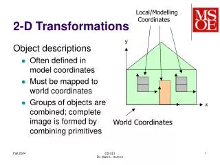
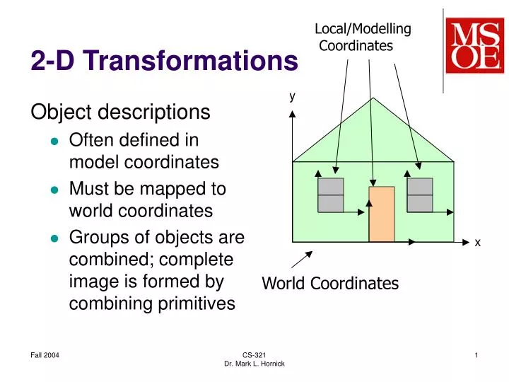
2-D Transformations. Local/Modelling Coordinates. y. Object descriptions Often defined in model coordinates Must be mapped to world coordinates Groups of objects are combined; complete image is formed by combining primitives. x. World Coordinates. 2-D Transformations.

E N D
2-D Transformations Local/Modelling Coordinates y Object descriptions • Often defined in model coordinates • Must be mapped to world coordinates • Groups of objects are combined; complete image is formed by combining primitives x World Coordinates CS-321Dr. Mark L. Hornick
2-D Transformations Local/Modelling Coordinates y Problem statement: • Convert points from coordinates in one system to a second coordinate system x World Coordinates CS-321Dr. Mark L. Hornick
2-D Transformations • First, consider the case where two coordinate systems are offset by a pure translation • Definitions • v2 – vector from origin of coordinate system xy2 to a point on the object • has scalar components (v2x,v2y) • v1 – vector from origin of coordinate system xy1 to a point on the object • has scalar components (v1x,v1y) • p – vector from origin of coordinate system xy1 to the origin of xy2 • has scalar components (px,py) y1 y2 v2 v1 x2 p x1 CS-321Dr. Mark L. Hornick
2-D Transformations:Translation • Using vector math: • v1 = p + v2 • In terms of scalar components: • v1x = px + v2x • v1y = py + v2y • And conversely: • v2 = v1 – p • v2x = v1x - px • v2y = v1y - py y1 y2 v2 v1 x2 p x1 CS-321Dr. Mark L. Hornick
y2 v2 x2 2-D Transformations:Rotation • Now consider the case of a pure rotation of one coordinate system with respect to the other • A simple case is rotation by 180 degrees • In this case, vectors v1 and v2 are coincident (they lie on top of each other), but they have opposite sense, that is: • v1 = -v2 • In terms of scalar components: • v1x = - v2x • v1y = - v2y v1 x1 y1 y2 v2 v1 x2 x1 y1 CS-321Dr. Mark L. Hornick
y2 y2 x2 x2 2-D Transformations:Rotation x1 • Next, consider the general case of a pure rotation of one coordinate system with respect to the other, but through an arbitrary angle v1 v2 x1 v2 v1 y1 CS-321Dr. Mark L. Hornick
y2 y2 x2 x2 2-D Transformations:Rotation x1 • Using trigonometry, it can be shown that: • In terms of scalar components: • v1x = v2xcos - v2y sin • v1y = v2ycos + v2xsin • In vector terms: • v1 = v2cos + (-v2y,v2y)sin • But what vector is (-v2y,v2y)? • It can be shown that v1 v2 x1 v2 v1 y1 CS-321Dr. Mark L. Hornick
y2 y2 x2 x2 2-D Transformations:Rotation x1 • Instead of using vector representation, these equations can also be cast in matrix form: v1 v2 x1 v2 v1 y1 CS-321Dr. Mark L. Hornick
y2 y2 x2 x2 2-D Transformations:Rotation x1 • Now that we have v1 in terms of v2, how do we express v2 in terms of v1 ? • Where R()-1 is the inverse of R() v1 v2 x1 v2 v1 y1 CS-321Dr. Mark L. Hornick
y2 y2 x2 x2 2-D Transformations:Rotation x1 • To express v2 in terms of v1, we can think of xy1 rotated through a negative angle v1 v2 x1 v2 v1 y1 CS-321Dr. Mark L. Hornick
y2 y2 x2 x2 2-D Transformations:Rotation x1 • So the inverseR()-1 is R(-) • Note also that the inverse R()-1is simply the transpose of R(-) since the off-diagonal elements are swapped • This is a property of special matrices called orthonormal matrices; Rotation matrices are orthonormal • This makes it easy to find the inverse of a rotation matrix v1 v2 x1 v2 v1 y1 CS-321Dr. Mark L. Hornick
y2 x2 Combining Rotation and Translation • The case of combined rotation and translation can be deconstructed into a pure rotation followed by a pure translation. • The pure rotation transforms vector v2 from coordinate frame xy1 to vector v*2 in frame xy*2 • The following pure translation transforms v*2 from frame xy*2 into vector v1 in frame xy1 y*2 x1 v1 v2 x*2 p y1 CS-321Dr. Mark L. Hornick
y2 x2 Combining Rotation and Translation • The equations that describe this transformation are just the combination of those we have already seen: y*2 x1 v1 v2 x*2 p y1 CS-321Dr. Mark L. Hornick
y2 x2 Combining Rotation and Translation • This equation can be recast using a mathematical trick: • This is called a 3x3 homogeneous transformation matrix T(,p) y*2 x1 v1 v2 x*2 p y1 CS-321Dr. Mark L. Hornick
y2 x2 Combining Rotation and Translation • T(,p) can be expressed in terms of submatrices as • The inverse of T(,p) is given by y*2 x1 v1 v2 x*2 p y1 CS-321Dr. Mark L. Hornick