Download
1 / 71
770 likes | 1.15k Views
Differential and precision GPS surveying for sub-meter and centimeter accuracy Feb 2007 Dr. Gary Oppliger. GPS navigation, mapping and surveying. Uses of GPS. Location - determining a basic position Navigation - getting from one location to another Mapping - creating maps of the world

E N D
Differential and precision GPS surveying for sub-meter and centimeter accuracyFeb 2007 Dr. Gary Oppliger
Uses of GPS • Location - determining a basic position • Navigation - getting from one location to another • Mapping - creating maps of the world • Tracking - monitoring the movement of people and things • Timing - providing precise timing to any location.
Differential GPS Differential GPS requires the simultaneous operation of two receivers. • A stationary receiver at a known position provides positional error correction to the roving or working receiver. • The corrections are transmitted in real-time by radio link or preformed by post survey processing.
Dual Freq. code and phase DGPS technique • Distance based on carrier signal phase
After this lecture you should be able to answer these questions: • How are personal GPS receivers different from survey-grade GPS receivers? • What does a survey-grade GPS receiver measure and record for each data epoch? • What is differential GPS post processing? • How is distance accuracy related to the length of the analyzed waveform? • What is carrier frequency cycle ambiguity and how can it be resolved? • How are various GPS surveys designed?
How GPS works The GPS system uses precisely timed radio transmissions from satellites with accurately known orbits to estimate locations of GPS receivers on earth. By very accurately “measuring” a GPS receiver’s distance (wave travel time) from 3 or 4 satellites its position can be triangulated.
Triangulation The measured distance between a satellite and GPS receiver defines a sphere centered on the satellite. The receiver could be located any where on that sphere.
Triangulation The intersections of three such spherical surfaces associated with three satellites cross at only two points, only one of which is generally physically possible. This point is displayed as the location of the GPS receiver.
GPS DOP - dilution of precision • PDOP: Position DOP, an overall measure of loss of precision. • HDOP: Horizontal DOP. • VDOP Vertical DOP. • TDOP: Time DOP. • GDOP: Geometric DOP both position and time.
GPS DOP - dilution of precision • In general, DOP values below 4 indicate excellent observation conditions; values above 7 indicate poor conditions. • In general, the vertical error (for estimated elevations) are two to three times greater than the horizontal error.
Satellite visibility planning Note absence of satellites in northern sky
Satellite visibility planning Screen from : GPSurvey Plan Down to minimum of 4 satellites PDOP above maximum of 7
Satellite visibility planning Ideal satellite visibility for one a hour interval 2 - 3 pm. Note: 15 degree azimuth satellite visibility mask level
Return to Triangulation The intersections of three such spherical surfaces associated with three satellites cross at only two points, only one of which is generally physically possible. This point is displayed as the location of the GPS receiver.
Distance to the satellites The “travel time” of the radio signal from the satellite to receiver times the speed-of-light (with some adjustments for the ionosphere) provides the distance.
Distance to the satellites Travel time determination requires precise clock synchronization in the satellites and GPS receiver. • The satellites use precise atomic clocks synchronized to a master earth based clock. • A GPS receiver is able to calculate the time from the position triangulation equations by observing a forth satellite.
The accuracy of distance estimates are linked to the length of the analyzed waveform Psuedo-Random-Sequence “bit” 1 Mhz 300 m PRS 1/100 “bit” fraction 3 m Carrier waveform 1.227 Mhz 24.4 cm Carrier waveform phase (36 degrees) 1/10 cycle 2.4 cm Waveform cycle rate length
Determining satellites orbits Satellite orbital tracks (or ephemeris) must be known to a few centimeters. • The DoD monitors the satellites' altitude, position and speed for "ephemeris" errors caused by gravitational and solar effects.
Receiving satellite orbit data • This information is relayed to the satellite which then broadcasts these corrections along with timing information in a system "data message“ that is 30 seconds long.
Receiving satellite orbit data • This data message (the almanac) contains the current orbital locations of all of the satellites. • Until this message is successfully received, the GPS receiver can not determine its position.
Doppler frequency • It very important to know each satellites location so the GPS receiver can continuously adjust its tuning filters to match the amount of radio frequency Doppler shift. • The first received satellites are typically those directly overhead, as they exhibits minimal Doppler frequency shift
Satellite radio signals • Two carrier frequencies used by GPS are 1227.60 MHz (L1) and 1575.42 MHz (L2). • On the L1, frequency a Coarse/Acquisition (C/A) Code is transmitted consisting of 1023 binary pseudo-random codes at a bit rate of 1.023 MHz.
Pseudo-random codes • By using repeated, long pseudo-random codes, GPS signals can be very low power and can still be picked up by an antenna a few centimeters across.
Derived from Blewitt 1997 Pseudo-random codes • The GPS receiver adjusts and compares its internally generated pseudo-random code with the received signal until its precise frequency and time shift are found. • This process is called locking onto the signal and can take several minutes.
From Blewitt 1997 Pseudorange estimation
Dual Freq. code and phase DGPS technique • Distance based on carrier signal phase • Phase ambiguity resolution (solution)
Distance based on carrier phase • Two carrier frequencies used by GPS are 1227.60 MHz (L1) and 1575.42 MHz (L2). • On the L1, frequency a Course/Acquisition (C/A) Code is transmitted consisting of 1023 binary pseudo-random codes at a bit rate of 1.023 MHz.
Distance based on carrier phase From Blewitt 1997
Distance based on carrier phase • Identifying the cycle being received allows for about 20 cm accuracy. L1 wave length is 24.4 cm L2 wave length is 19 cm.
Distance based on carrier phase • Identifying the phase position in a cycle allows sub-centimeter accuracy. ~24 cm Figure after Blewitt 1997
For each data epoch a survey-grade GPS receiver measures and records: • Carrier cycle count for each satellite an frequency L1, L2 • Relative carrier phase shifts between all satellite signals • Estimated time of data epoch
Ambiguity resolution • Without knowledge of the particular cycle being observed thousands of positional solutions are possible, but with enough data it is possible demonstrate one solution is far more probable.
Ambiguity resolution • The essence of sub-meter GPS surveying is to acquire enough data sets (or epochs) to unquestionably resolve the cycle ambiguities. • If enough quality data is not acquired the measurement fails to be resolved; and will have to be re-surveyed.
Ambiguity resolution • Strategies for maximizing chances of resolving ambiguities in static GPS surveys: • Keep baselines short • Dual-frequency for more observed parameters • Adequate length observation session • Minimize interference from multipath by good selection of sites, observing at night. • Observe as many satellites as possible to ensure good receiver-satellite geometry.
Ambiguity resolution • Once the cycle and phase ambiguities are resolved for a station that “lock” may be maintained by uninterrupted observation (measuring) as you move between stations. • Referred to as Stop-n-Go Kinematic. • On-the-fly ambiguity resolution may be utilized. • Reduces static time required at each station.
Ambiguity resolution • The design and execution of every efficient post-processing GPS survey should balance the cost of acquiring enough data at each station to resolve ambiguities against the cost of repeating a failed measurement.
Multipath interference • Multipath interference refers to satellite signal reflections from objects around the antenna. • This is identical to TV signal ghosting effects. • The receiver may confuse the ghost with the direct signal and get the travel time wrong. • At a minimum the quality of the data is lowered.
Multipath interference • Reduce effects by: • Good site selection i.e., away from buildings, rock faces and trees. • Use of a choke ring antenna – stops reflections from the ground. • Record for a longer period of time. • Survey a problem site by a non-GPS method. • Use most advanced GPS receivers.
Dual frequency correction of ionosphere propagation delays • Precision GPS surveying requires accurate estimates of ionosphere produced signal time delays. • The ionosphere causes EM wave dispersion, which means different frequencies travel at different speeds. • By observing the relative differences in the L1 qnd L2 travel times from a single satellite the total delay can be estimated and corrected.
Short and long baseline differential GPS methods for sub-decimeter <10 cm accuracy • Short baseline applies for 10 kms or less. • requires observation times of 10 to 20 minutes. • Long baseline applies for 20 km – 200 km or more. • Requires observation times of 4 hours to a day. Note the jump in the required observations times.
Short baseline DGPS (< 10 km)sub-decimeter accuracy • Real-time kinematic • Radio-link is necessary • Allows +/- 10 cm stakeout of planned points • Good sky view required to maintain phase lock • The quality of the position solution is known at all times. • No post processing required – saves time.
Short baseline DGPS (< 10 km)sub-decimeter accuracy Post processing field methods • Fast static - 10 – 20 minutes per station • Kinematic - initialize at a point then survey • Stop-n-Go kinematic - combines both
Short baseline DGPS (< 10 km)sub-decimeter accuracy • Post processing advantages / disadvantages • Post processing takes extra time. • Quality of position solutions not known until post processed. • Delayed processing allows use of precise ephemeris for better results.
Short baseline DGPS (< 10 km) • Accuracy 1 - 30 cm (x,y,z) depends on: • Static occupation time • Length of baseline • Processing methods Accuracy examples: • -/+15 cm (3 sigma/ 99%) requires 15 minutes for 10 km baseline. • -/+2 cm (3 sigma/ 99%) requires several hours
Long baseline DGPS (> 20 km)sub-decimeter accuracy • Post processing methods • Static long occupations > 2 hours • Kinematic - special applications only • Real-time kinematic methods • Not practical at sub-decimeter accuracy • Practical at sub-meter accuracy
Long baseline DGPS (>20 km) • Accuracy 1 - 30 cm (x,y,z) depends on: • Static occupation time • Length of baseline • Processing methods Accuracy examples: • -/+15 cm (3 sigma/ 99%) requires 2 hours • -/+1 cm (3 sigma/ 99%) requires several days
Long baseline DGPS (> 20 km) • Conclusion: Static methods can work well at the +/- 5 cm level on baselines 200 km or longer with just 4 hours of data if the data is processed by OPUS.
Geodetic control resources National Geodetic Survey (NGS) website • Survey control monument datasheets • Coordinate conversion tools • GPS reference station network (CORS) • Long baseline GPS processing service • GPS data format conversion utilities • ITRF crustal motion coordinate models • Geoid models