Download

1 / 17
170 likes | 300 Views
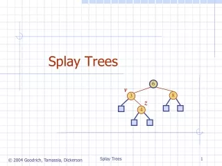
6. v. 8. 3. z. 4. Splay Trees. all the keys in the blue region are 20. all the keys in the yellow region are 20. Splay Trees are Binary Search Trees. ( § 9.3). (20,Z). note that two keys of equal value may be well-separated. BST Rules: entries stored only at internal nodes

E N D
6 v 8 3 z 4 Splay Trees Splay Trees
all the keys in the blue region are 20 all the keys in the yellow region are 20 Splay Trees are Binary Search Trees (§ 9.3) (20,Z) note that two keys of equal value may be well-separated • BST Rules: • entries stored only at internal nodes • keys stored at nodes in the left subtree of v are less than or equal to the key stored at v • keys stored at nodes in the right subtree of v are greater than or equal to the key stored at v • An inorder traversal will return the keys in order (10,A) (35,R) (14,J) (7,T) (21,O) (37,P) (1,Q) (8,N) (36,L) (40,X) (1,C) (10,U) (5,H) (7,P) (2,R) (5,G) (6,Y) (5,I) Splay Trees
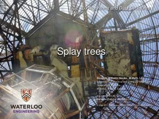
(20,Z) (10,A) (35,R) (14,J) (7,T) (21,O) (37,P) (1,Q) (8,N) (36,L) (40,X) (1,C) (10,U) (5,H) (7,P) (2,R) (5,G) (6,Y) (5,I) Searching in a Splay Tree: Starts the Same as in a BST • Search proceeds down the tree to found item or an external node. • Example: Search for time with key 11. Splay Trees
(20,Z) (10,A) (35,R) (14,J) (7,T) (21,O) (37,P) (1,Q) (8,N) (36,L) (40,X) (1,C) (10,U) (5,H) (7,P) (2,R) (5,G) (6,Y) (5,I) Example Searching in a BST, continued • search for key 8, ends at an internal node. Splay Trees
Splay Trees do Rotations after Every Operation (Even Search) • new operation: splay • splaying moves a node to the root using rotations • right rotation • makes the left child x of a node y into y’s parent; y becomes the right child of x • left rotation • makes the right child y of a node x into x’s parent; x becomes the left child of y y x a right rotation about y a left rotation about x y T1 x T3 x y T3 T1 T2 T2 y T1 x T3 T3 T2 T1 T2 (structure of tree above x is not modified) (structure of tree above y is not modified) Splay Trees
“x is aleft-left grandchild” means x is a left child of its parent, which is itself a left child of its parent • p is x’s parent; g is p’s parent Splaying: start with node x is x a left-left grandchild? is x the root? zig-zig yes stop right-rotate about g, right-rotate about p yes no is x a right-right grandchild? zig-zig is x a child of the root? no left-rotate about g, left-rotate about p yes is x a right-left grandchild? yes zig-zag is x the left child of the root? left-rotate about p, right-rotate about g no yes is x a left-right grandchild? zig zig zig-zag yes right-rotate about p, left-rotate about g right-rotate about the root left-rotate about the root yes Splay Trees
Visualizing the Splaying Cases zig-zag x z z z y y T4 T1 y T1 T2 T3 T4 T4 x T3 x T2 T3 T1 T2 zig-zig y zig x T4 x T1 x y w T2 y z T3 w T1 T2 T3 T4 T3 T4 T1 T2 Splay Trees
(20,Z) (20,Z) (10,A) (35,R) (35,R) (8,N) x g (14,J) (7,T) (10,A) (21,O) (37,P) p (21,O) (37,P) (20,Z) (10,A) g (36,L) (40,X) (1,Q) (8,N) (36,L) (40,X) (35,R) (8,N) x (14,J) (14,J) (7,T) (7,T) (1,C) (21,O) (37,P) (10,U) (5,H) p (7,P) (1,Q) (1,Q) (36,L) (40,X) (2,R) (5,G) (1,C) (1,C) (10,U) (10,U) (5,H) (5,H) (7,P) (7,P) (6,Y) (5,I) (2,R) (2,R) (5,G) (5,G) (6,Y) (6,Y) (5,I) (5,I) Splaying Example g 1. (before rotating) p x • let x = (8,N) • x is the right child of its parent, which is the left child of the grandparent • left-rotate around p, then right-rotate around g 2. (after first rotation) 3. (after second rotation) x is not yet the root, so we splay again Splay Trees
(20,Z) (35,R) (8,N) x (8,N) x (10,A) (21,O) (37,P) (20,Z) (36,L) (40,X) (35,R) (10,A) (21,O) (37,P) (14,J) (14,J) (7,T) (7,T) (36,L) (40,X) (1,Q) (1,Q) (1,C) (1,C) (10,U) (10,U) (5,H) (5,H) (7,P) (7,P) (2,R) (2,R) (5,G) (5,G) (6,Y) (6,Y) (5,I) (5,I) Splaying Example, Continued • now x is the left child of the root • right-rotate around root 2. (after rotation) 1. (before applying rotation) x is the root, so stop Splay Trees
(20,Z) (20,Z) (40,X) (10,A) (35,R) (10,A) (14,J) (37,P) (7,T) (14,J) (7,T) (21,O) (37,P) (35,R) (1,Q) (8,N) (40,X) (20,Z) (1,Q) (8,N) (36,L) (40,X) (21,O) (36,L) (1,C) (10,U) (5,H) (7,P) (10,A) (37,P) (2,R) (5,G) (1,C) (10,U) (5,H) (7,P) (14,J) (35,R) (7,T) (6,Y) (5,I) (1,Q) (8,N) (21,O) (36,L) (2,R) (5,G) (1,C) (10,U) (5,H) (7,P) (6,Y) (5,I) (2,R) (5,G) (6,Y) (5,I) Example Result of Splaying before • tree might not be more balanced • e.g. splay (40,X) • before, the depth of the shallowest leaf is 3 and the deepest is 7 • after, the depth of shallowest leaf is 1 and deepest is 8 after first splay after second splay Splay Trees
Splay Tree Definition • a splay tree is a binary search tree where a node is splayed after it is accessed (for a search or update) • deepest internal node accessed is splayed • splaying costs O(h), where h is height of the tree – which is still O(n) worst-case • O(h) rotations, each of which is O(1) Splay Trees
Splay Trees & Ordered Dictionaries • which nodes are splayed after each operation? method splay node if key found, use that node if key not found, use parent of ending external node find(k) insert(k,v) use the new node containing the entry inserted use the parent of the internal node that was actually removed from the tree (the parent of the node that the removed item was swapped with) remove(k) Splay Trees
Amortized Analysis of Splay Trees • Running time of each operation is proportional to time for splaying. • Define rank(v) as the logarithm (base 2) of the number of nodes in subtree rooted at v. • Costs: zig = $1, zig-zig = $2, zig-zag = $2. • Thus, cost for playing a node at depth d = $d. • Imagine that we store rank(v) cyber-dollars at each node v of the splay tree (just for the sake of analysis). Splay Trees
y zig T4 x x w T3 y w T1 T2 T3 T4 T1 T2 Cost per zig • Doing a zig at x costs at most rank’(x) - rank(x): • cost = rank’(x) + rank’(y) - rank(y) - rank(x) < rank’(x) - rank(x). Splay Trees
zig-zag x z z zig-zig z T4 y y T1 y T1 T2 T3 T4 T4 x T3 x T2 T3 T1 T2 x T1 y T2 z T3 T4 Cost per zig-zig and zig-zag • Doing a zig-zig or zig-zag at x costs at most 3(rank’(x) - rank(x)) - 2. • Proof: See Proposition 9.2, Page 440. Splay Trees
Cost of Splaying • Cost of splaying a node x at depth d of a tree rooted at r: • at most 3(rank(r) - rank(x)) - d + 2: • Proof: Splaying x takes d/2 splaying substeps: Splay Trees
Performance of Splay Trees • Recall: rank of a node is logarithm of its size. • Thus, amortized cost of any splay operation is O(log n). • In fact, the analysis goes through for any reasonable definition of rank(x). • This implies that splay trees can actually adapt to perform searches on frequently-requested items much faster than O(log n) in some cases. (See Proposition 9.4 and 9.5.) Splay Trees