I. Lagrangians Why we love symmetries, even to the point of seemingly

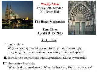
1. Weekly Mass Friday, 4:00 Service 201 Brace Hall The Higgs Mechanism Dan Claes April 8 & 15, 2005 An Outline I. Lagrangians Why we love symmetries, even to the point of seemingly imagining them in all sorts of new non-geometrical spaces. II. Introducing interactions into Lagrangians: SU(n) symmetries III. Symmetry Breaking Where’s the ground state? What the heck are Goldstone bosons?

2. The precise dynamical behavior of a system of particles can be inferred from the Lagrangian equations of motion derived from the Lagrange function: here for a classical systems of mass points Extended to the case of continuous (wave) function(s) “The Lagrangian” m an explicit function only of the dynamical variables of the field components and their derivatives Euler-Lagrange equation

3. m • Does not depend explicitly on spatial coordinates (absolute positions) • the “Ruler Postulate” translation invariance - otherwise would violate relativistic invariance Conservation of Linear Momentum! • Does not depend explicitly on t (absolute time) time translation invariance Conservation of Energy! • Similarly its invariance under spacial rotations - guaranteesConservation of Angular Momentum!

4. m • The value of , i.e., at , must depend only on value(s) of • and its derivatives at . - no “non-local” terms which, in general, create problems in causality and with non-real physics quantities - non-local terms never appear in any Standard Model field theory though often considered in theories seeking to extend field theory “beyond the Standard Model” THINK: wormholes and time travel • For linear wave equations need terms at least quadratic in • and - To generate differential equations not higher than 2nd order restrict terms to factors of the field components and their 1st derivative - note: renormalizability demands no higher powers in the fields than and than n = 5.

5. m • L should be real(field operators Hermitian) - guarantees the dynamical variables (energy, momentum, currents) are real. • L should be relativistically invariant - so restrictive is this requirement, it guarantees the derived equations of motion are automatically Lorentz invariant

6. Real Scaler Field £ £ £ the simplest Lagrangian with (xm) and m  dependence is from which  / - m[ / (m) ] = 0 yields the (hopefully) familiar Klein-Gordon equation! 1920 E. Schrödinger O. Klein W. Gordon From the starting point for a relativistic QM equation: together with the quantum mechanical prescriptions

7. ₤ ₤ Matter fields (like the QM wave function of an electron) are known only up to a phase factor a totally non-geometric attribute If we choose, we can write this as or or

8. ₤ ₤ ₤ ₤ ₤ Then treating  and* as independent fields, we find field equations  / - m[ / (m) ] = 0  /*-m[ / (m*)] = 0 two real fields describing particles of identical mass There’s a new symmetry hidden here:the Lagragian is completely invariant under any arbitrary rotation in the complex plane or

9. ₤ ₤ ₤ ₤ ₤ ₤ ₤ ₤ ₤ ₤ ₤ ₤ ₤ For an infinitesimally small rotation = 0 satisfying the continuity equation! and changing sign with f f* a conserved 4-vector a charged current density

10. ₤ This is easily extended to 3 (or more) related, but independent fields for example: allows us to consider a class of unitary transformations wider than the single-phase U(1)

11. Vector Field £ Spin-1 particles the field now has 4 components γ, g, W, Z Though has all the 4-vectors, tensors contracted energy is not positive definite unless we impose a restriction i.e., only 3 linearly independent components This is equivalent to replacing the 1st term with the invariant expression the (hopefully still) familiar Klein-Gordon equation!

12. Dirac Field Spin- ½ particles this field includes 4 independent components in spinor space e, m, quarks LDIRAC Dirac’s equation with a current vector:

13. These have been single free particle Lagrangians We might expect a realistic Lagrangian that involves systems of particles L(r,t) = LVector + LDIRAC but each term describes free non-interacting particles describes photons describes e+e-objects need something like: L +L INT But what should an interaction term look like? How do we introduce the interactions they experience? Again: a local Hermitian Lorentz-invariant construction of the various fields and their derivatives reflecting any additional symmetries the interaction has been observed to respect The simplest here would be a bilinear form like:

14. Or consider this: Our free particle equations of motion were all homogeneous differential equations. When the field is due to a source, like the electromagnetic (photon!) field you know you need to make the eq. of motion inhomogeneous: charged 4-current density and would do the trick! exactly the proposed bilinear form! Dirac electron current

15. Just crack open Jackson: A charge interacts with a field through: current-field interactions the fermion (electron) the boson (photon) field from the Dirac expression for J particle field antiparticle (hermitian conjugate) field

16. Now let’s look back at the FREE PARTICLE Dirac Lagrangian LDirac=iħcgm  mc2 Dirac matrices Dirac spinors (Iso-vectors, hypercharge) Which is OBVIOUSLY invariant under the transformation ei (a simple phase change) because  e-i and in all  pairings this added phase cancels! This one parameter unitary U(1) transformation is called a“GLOBAL GAUGE TRANSFORMATION.”

17. What if we GENERALIZEthis? Introduce more flexibility to the transformation? Extend to: but still enforce UNITARITY? eia(x) LOCAL GAUGE TRANSFORMATION Is the Lagrangian still invariant? LDirac=iħcgm  mc2 (ei(x)) = i((x)) + ei(x)() So: L'Dirac = -ħc((x))gm +iħce-i(x)gm()e+i(x) mc2

18. L'Dirac = -ħc((x))gm+iħcgm() mc2 LDirac For convenience (and to make subsequent steps obvious) define: -ħc q (x)  (x) then this is re-written as L'Dirac = +qgm()+LDirac recognize this????

19. L'Dirac = +qgm()+LDirac If we are going to demand the complete Lagrangian be invariant under even such a LOCAL gauge transformation, it forces us to ADD to the “free” Dirac Lagrangian something that can ABSORB (account for) that extra term, i.e., we must assume the full Lagrangian HAS TO include a current-field interaction: L=[iħcgmmc2]-(qgm)Am and that defines its transformation under the same local gauge transformation

20. L=[iħcgmmc2]-(qgm)Am • We introduced the same interaction term moments ago • following electrodynamic arguments (Jackson) • the form of the current density is correctly reproduced • the transformation rule • Am' = Am +  l • is exactly (check your Jackson notes!) • the rule for GAUGE TRANSFORMATIONS • already introduced in e&m! • The exploration of this “new”symmetry shows that for an SU(1)- • invariant Lagrangian, the freeDirac Lagrangain is “INCOMPLETE.” • If we chose to allow gauge invariance, it forces to introduce • a vector field (here that means Am) that “couples” to.

21. We can generalize our procedures into a PRESCRIPTION to be followed, noting the difference between LOCAL and GLOBAL transformations are due to derivatives:   /=  [e+iq/ħc] = e+iq/ħc forU(1)this is a 1×1unitary matrix (just a number) the extra term that gets introduced If we replace every derivative in the original free particle Lagrangian with the “co-variant derivative” D= + iA g ħc then the gauge transformation ofAwill cancel the term that appears through (D)/= e-iq/ħcD i.e. restores the invariance of L

22. SU(3)color symmetry of strong interactions This same procedure, generalized to symmetries in new spaces SU(3) “rotations” occur in an 8-dim “space” 8 3x3 “generators” 3-dimensional matrix formed by linear combinations of 8 independent fundamental matrices 8-dim vector Demanding invariance of the Lagrangian under SU(3) rotations introduces the massless gluon fields we believe are responsible for the strong force. The field is assumed to exist in any of 3 possible independent colorstates

23. in an effort to explain decays: THEN e _ e d d u ?? u d proton neutron decay u e _  e ?? muon decay  + pion hadron decays involve the transmutation of individual quarks u d _ ?? 

24. as well as the observed inverse of some of these processes: d neutrino capture by protons u d d u u e+ _ ?? e e e ??   neutrino capture by muons

25. in terms of the gauge model of photon-mediated charged particle interactions e- e- p p  ??? p e- n e required the existence of 3 “weakons” : W +, W -, Z me e+ W + m+ d e+ W +? W -? u e ue e- W - d

26. SU(2) electro-weak symmetry 1 2 u d e e- “Rotational symmetry”within weakly coupled left-handed isodoublet states introduces 3 weakons: W+, W-, Z and an associated weak isospin “charge” L L

27. This SU(2) theory then     L=[iħcgmmc2]- F F-(ggm )·Gm 1 4  2 describes doublet Dirac particle states in interaction with 3 massless vector fields Gm (think of somethinglike the-fields,A)   This followed just by insisting on local SU(2) invariance! In the Quantum Mechanical view:    2 • These Dirac fermions generate 3 currents, J = (g  ) • These particles carry a “charge” g, which • is the source for the 3 “gauge” fields

28. so named because unlike the PROMPT processes The Weak Force  qg e+ e- _ which seem instantaneous rg e+ e-  qr    or the electromagnetic decay: which involves a 10-17 sec lifetime path length (gap) in photographic emulsions mere nm! weak decays are “SLOW” processes…the particles involved: , ±,  are nearly “stable.” 10-6 sec 700 m pathlengths 887 sec 10-8 sec +++ 7 m pathlengths and their inverse processes: scattering or neutrino capture are rare small probability of occurrence (small rates…small cross sections!).

29. Such “small cross section” seemed to suggest a SHORT RANGE force…weaker with distance compared to the infinite range of the Coulomb force or powerful confinement of the color force This seems at odds with the predictions of ordinary gauge theory in which the VECTOR PARTICLES introduced to mediate the forces like photons and gluons are massless. This means the symmetry cannot be exact. The symmetry is BROKEN.

30. Some Classical Fields The gravitational field around a point source (e.g. the earth) is a scalar field An electric field is classical example of a vector field: effectively 3 independent fields

31. Once spin has been introduced, we’ve grown accustomed to writing the total wave function as a two-component “vector” ψ↑(x,y,z) ψ↓(x,y,z) Ψ(x,y,z,t;ms) = Ψ = e-iEt/ħψ(x,y,z)g(ms) time- dependent part spatial part spin space α β Ψ = e-iEt/ħR(r)S(θ)T(φ)g(ms) Yℓm(θ,φ) for a spherically symmetric potential But spin is 2-dimensional only for spin-½ systems. Recognizing the most general solutions involve ψ/ψ* (particle/antiparticle) fields, the Dirac formalism modifies this to 4-component fields! The 2-dim form is better recognized as just one fundamental representation of angular momentum.

32. That 2-dim spin-½ space is operated on by or more generally by The SU(2) transformation group (generalized “rotations” in 2-dim space) is based on operators: U “generated by” traceless Hermitian matrices

33. What’s the most general tracelessHERMITIAN 22 matrices? a-ib c a+ib -c and check out: c a-ib a+ib -c 0 1 1 0 0 -i i 0 1 0 0 -1 = a +b +c

34. SU(3) FOR What’s the form of the most general traceless HERMITIAN 3×3 matrix? a1-ia2 a3 a4-ia5 Diagonal terms have to be real! Transposed positions must be conjugates! a1+ia2 a6-ia7 a4+ia5 a6+ia7 Must be traceless! 0 0 1 0 0 0 1 0 0 0 -i 0 i 0 0 0 0 0 0 1 0 1 0 0 0 0 0 = a1 +a2 +a3 +a4 +a3+a6 +a7 +a8 0 0 0 0 0 1 0 1 0 0 0 0 0 0 -i 0 i 0 0 0 -i 0 0 0 i0 0

35. U(1) local gauge transformation (of simple phase) electrical charge-coupled photon field mediates EM interactions SU(2) “rotations” occur in an 3-dim “space” e-ia·/2ħ three 2x2 matrix operators 3 independent parameters 3 simultaneous gauge transformations 3 vector boson fields SU(3) “rotations” occur in an 8-dim “space” e-ia·/2ħ 8 3x3 operators 8 independent parameters 8 simultaneous gauge transformations 8 vector boson fields

36. Spontaneous Symmetry Breaking Englert & Brout, 1964 Higgs 1964, 1966 Guralnick, Hagen & Kibble 1964 Kibble 1967 The Lagrangian& derived equations of motion for a system possess symmetries which simply do NOT hold for a specific ground state of the system.(The full symmetry MAY be re-stored at higher energies.) • (1) A flexible rod under longitudinal compression. • (2) A ball dropped down a flask with a convex bottom. • Lagrangian symmetric with respect to • rotations about the central axis • once force exceeds some critical value it must buckle • sideways forming an arc in SOME arbitrary direction • Although one direction is chosen, the complete set of all possible final shapes DOES show the full symmetry.

37. What is the GROUND STATE? lowest energy state What does GROUND STATE mean in Quantum Field Theory? Shouldn’t that just be the vacuum state?|0  which has an compared to 0. Fields are fluctuations about the GROUND STATE. Virtual particles are created from the VACUUM. The field configuration of MINIMUM ENERGY is usually just the obvious  0 (e.g. out of  away from a particle’s location)

38. Following the definition of the discrete classical L = T -V we separate out the clearly identifiable “kinetic” part L = T( ∂f ) – V(f ) For the simple scalar field considered earlier V(f)=½m2f 2 is a 2nd-order parabola: V(f) The f → 0 case corresponds to a stable minimum of the potential. Quantization of the field corresponds to small oscillations about the position of equilibrium there. f Noticein this simple modelV is symmetric to reflections off -f

39. Obviously as 0 there are no intereactions between the fields and we will have only free particle states. And as(or in regions where)  0 we have the empty state | 0  representing the lowest possible energy state and serving as the vacuum. The exact numerical value of the energy content/density of | 0  is totally arbitrary…relative. We measure a state’s or system’s energy with respect to it and usually assume it is or set it to 0. What if the EMPTY STATE did NOT carry the lowest achievable energy? = We will call 0||0 = vev the “vacuum expectation value” of an operator state.

40.  √λ  √λ  √λ Now let’s consider a model with a quartic (“self-interaction”) term: £=½+½2¼4 Such models were 1st considered for observed interactions like with this sign, we’ve introduced a term that looks like an imaginary mass (in tachyon models) +-→ 00 V(f) = -½2 + ¼4 =-½2(- ½λ2) Now the extrema at f = 0 is a local maximum! - Stable minima atf0= ± a doubly degenerate vacuum state The depth of the potential at f0 is

41.  √λ  √λ V(f) = -½2 + ¼4 - A translation f(x)→ u(x) ≡ f(x) – f0 selects one of the minima by moving into a new basis redefining the functional form of f in the new basis (in order to study deviations in energy from the minimum f0) V(f) = V(u+f0) = -½(u+f0)2 + ¼ (u+f0)4 = V0+u2+ √ u3+ ¼u4 plus new self- interaction terms The observable field describes particles of ordinary massm/2. energy scale we can neglect

42. Complex Scalar field £=½+½¼ Note:OBVIOUSLY globally invariant under U(1) transformations   ei £=½11 + ½22 ½12+22 ¼12+22  1 2 Which is ROTATIONALLY invariant under SO(2)!! Our Lagrangian yields the field equation: 1 + 12+ 112+22  = 0 or equivalently 2 + 22+ 212+22  = 0 some sort of interaction between the independent states

43. Lowest energy states exist in this circular valley/rut of radius v =  2  1 This clearly shows the U(1)SO(2) symmetry of the Lagrangian But only one final state can be “chosen” Because of the rotational symmetry all are equivalent We can chose the one that will simplify our expressions (and make it easier to identify the meaningful terms) shift to the selected ground state expanding the field about the ground state:1(x)=+(x)

44. Scalar (spin=0) particle Lagrangian L=½11 + ½22 ½12+22 ¼12+22  with these substitutions: v = L=½ + ½ ½2+2v+v2+2  ¼2+2v+v2+2  becomes L=½ + ½ ½2+ 2 v ½v2 ¼2+2 ¼22+22v+v2 ¼2v+v2

45. L=½ + ½ ½(2v)2 v2+2¼2+2  + ¼v4 ½  ½(2v)2 Explicitly expressed in real quantities  and v this is now an ordinary mass term!  “appears” as a scalar (spin=0) particle with a mass ½  “appears” as a massless scalar There is NO mass term!

46. Of course we want even this Lagrangian to be invariant to LOCAL GAUGE TRANSFORMATIONS D=+igG Let’s not worry about the higher order symmetries…yet… free field for the gauge particle introduced Recall: F=G-G L= [-v22] + [  ] + [ FF+ GG] -gvG 1 2 g2v2 2 1 2 -1 4 g2 2 +{ gG[-] + [2+2v+2]GG  4  2 1 2 - [4v(3+2) + [ v4] + [4+222+ 4] and many interactions between  and  which includes a numerical constant v4 4

47. The constants , v give the coupling strengths of each                  

48. which we can interpret as: a whole bunch of 3-4 legged vertex couplings massless scalar  free Gauge field with mass=gv scalar field  with L = -gvG + + + But no MASSLESS scalar particle has ever been observed  is a ~massless spin-½ particle is a massless spin-1particle spinless,have plenty of mass! plus - gvG seems to describe G • Is this an interaction? • A confused mass term? • G not independent? ( some QM oscillation between mixed states?)  Higgs suggested:have not correctly identified the PHYSICALLY OBSERVABLE fundamental particles!

49. RememberLisU(1)invariant - rotationally invariant in , (1, 2) space – i.e. it can be equivalently expressed under any gauge transformation in the complex plane Note: or /=(cos + isin )(1 + i2) =(1cos-2sin ) + i(1sin+ 2cos) With no loss of generality we are free to pick the gaugea , for example, picking: /2  0 and/ becomes real!

50. ring of possible ground states equivalent to rotating the system by angle - 2  1  (x) (x) = 0