Download
1 / 134
1.38k likes | 1.57k Views
Packet Scheduling/Arbitration in Virtual Output Queues and Others. Key Characteristics in Designing Internet Switches and Routers. Scalability in terms of line rates Scalability in terms of number of interfaces (port numbers). Switch/Router Architecture Comparison.

E N D
Packet Scheduling/Arbitration in Virtual Output Queuesand Others
Key Characteristics in Designing Internet Switches and Routers • Scalability in terms of line rates • Scalability in terms of number of interfaces (port numbers)
Switch/Router Architecture Comparison http://www.lightreading.com/document.asp?doc_id=47959
Head-of-Line Blocking Blocked! Blocked!
Crossbar Switches: Virtual Output Queues • Virtual Output Queues: • At each input port, there are N queues – each associated with an output port • Only one packet can go from an input port at a time • Only one packet can be received by an output port at a time • It retains the scalability of FIFO input-queued switches (no memory bandwidth problem) • It eliminates the HoL problem with FIFO input Queues
VOQs: How Packets Move VOQs Scheduler
Scheduler Crossbar Scheduler in VOQ Architecture • Memory b/w=2R • Can be quite complex!
Question: do more lanes help? • Answer: it depends on the scheduling VOQs with Bad Scheduling Head of Line Blocking Good Scheduling? Ayalon: depends on traffic matrix…
Crossbar Scheduler in VOQ Architecture Which packets I can send during each configuration of the crossbar
Cell Data Port Processor Port Processor Crossbar optics optics LCS Protocol LCS Protocol optics optics Request Grant/Credit Switch core architecture Port #1 Scheduler (Like the Processor of A Computer) Port #256
Basic Switch Model S(n) L11(n) A11(n) 1 1 D1(n) A1(n) A1N(n) AN1(n) DN(n) AN(n) N N ANN(n) LNN(n)
Occupancy L11(n) LNN(n) Some definitions 3. Queue occupancies:
Some possible performance goals When traffic is admissible
VOQ Switch Scheduling • The VOQ switch scheduling can be represented by a bipartite graph • The left-hand side nodes of the bipartite graph are the input ports • The right-hand side nodes of the bipartite graph are the output ports • The edges between the nodes are requests for packet transmission between input ports and output ports. A 1 2 B 3 C 4 D 5 E 6 F
Maximum size bipartite match • Intuition: maximizes instantaneous throughput L11(n)>0 Maximum Size Match LN1(n)>0 Bipartite Match “Request” Graph
Network flows and bipartite matching Finding a maximum size bipartite matching is equivalent to solving a network flow problem with capacities and flows of size “1”. A 1 2 B Sink t Source s 3 C 4 D 5 E 6 F
10 10 10 1 10 1 10 1 Network Flows a c Source s Sink t b d • Let G=[V,E] be a directed graph with capacity cap(v,w) on edge [v,w]. • A flow is an (integer) function, f, that is chosen for each edge so that f(v,w) <= cap(v,w). • We wish to maximize the flow allocation.
10 10 10 1 10 1 10 1 a c 10, 10 Source s Sink t 10, 10 1 10, 10 10 1 10 b d 1 Flow is of size 10 A maximum network flow exampleBy inspection a c Source s Sink t b d Step 1:
Not obvious Maximum flow: a c 10, 9 Source s Sink t 10, 10 1,1 10, 10 1,1 10, 2 b d 10, 2 1, 1 Flow is of size 10+2 = 12 A maximum network flow example Step 2: a c 10, 10 Source s Sink t 10, 10 1 10, 10 1 10, 1 b d 10, 1 1, 1 Flow is of size 10+1 = 11
Ford-Fulkerson method of augmenting paths • Set f(v,w) = -f(w,v) on all edges. • Define a Residual Graph, R, in which res(v,w) = cap(v,w) – f(v,w) • Find paths from s to t for which there is positive residue. • Increase the flow along the paths to augment them by the minimum residue along the path. • Keep augmenting paths until there are no more to augment.
Example of Residual Graph a c 10, 10 10, 10 1 10, 10 s t 10 1 10 b d 1 Flow is of size 10 Residual Graph, R res(v,w) = cap(v,w) – f(v,w) a c 10 10 10 1 s t 10 1 10 b d 1 Augmenting path
Example of Residual Graph a c 10, 10 10, 10 1 10, 10 s t 10 1 10 b d 1 Flow is of size 10 Residual Graph, R res(v,w) = cap(v,w) – f(v,w) a c 10 10 10 1 s t 10 1 10 b d 1 Augmenting path
Example of Residual Graph Step 2: a c 10, 10 s t 10, 10 1 10, 10 1 10, 1 b d 10, 1 1, 1 Flow is of size 10+1 = 11 Residual Graph a c 10 s t 10 10 1 1 1 1 b d 9 1 9 Augmenting path
Example of Residual Graph Step 3: a c 10, 9 s t 10, 10 1, 1 10, 10 1, 1 10, 2 b d 10, 2 1, 1 Flow is of size 10+2 = 12 Residual Graph a c 10 s t 10 10 1 2 1 2 b d 8 1 8
f=4 12 12 a b 12 a b a b 16 20 16 20 16 20 9 4 9 s 10 t 9 4 7 s 10 t 4 s 10 t 7 7 4 13 4 4/13 4/4 4 11 4 4/11 c d 9 c d c d 7 An other Example: Ford-Fulkerson method find augmenting path p f=0 Gf G 12 a b 16 20 9 4 s 10 t 7 13 4 11 c d
f=4+12 12/12 12 a b a b 4 8 12/16 12/20 12 12 9 9 4 s 10 t 4 s 10 t 7 7 4 4/13 4/4 4 4 4/11 9 c d c d 7 An other Example: Ford-Fulkerson method find augmenting path p f=4 Gf G 12 12 a b a b 16 20 16 20 9 9 4 s 10 t 4 s 10 t 7 7 4 4/13 4/4 4 4 4/11 9 c d c d 7
f=16+7 12/12 12 a b a b 4 1 12/16 19/20 12 19 9 9 4 s 10 t 4 s 10 t 7/7 7 11 11/13 4/4 4 11/11 2 c d c d 11 An other Example: Ford-Fulkerson method find augmenting path p f=16 Gf G 12/12 12 a b a b 4 8 12/16 12/20 12 12 9 9 4 s 10 t 4 s 10 t 7 7 4 4/13 4/4 4 4 4/11 9 c d c d 7
An other Example: Ford-Fulkerson method find augmenting path p f=23 Gf G 12/12 12 a b a b 4 1 12/16 19/20 12 19 9 9 4 s 10 t 4 s 10 t 7/7 7 11 11/13 4/4 4 11/11 2 c d c d 11 No more augmenting path Maximum Flow is 23
S S S S S S S 10 10 0 10 10 10 10 10 10 9 9 9 9 9 9 9 9 10 10 10 10 0 9 9 9 9 9 9 9 9 10 10 10 0 10 10 10 10 10 T T T T T T T Input graph G Residual Graph Gr Flow graph Gf An example for Flow: Obvious solution Total flow = 10, Sub-optimal solution!
S S S S S S S S S S S S S 10 9 10 10 0 10 10 10 10 10 10 10 10 10 10 1 10 10 10 10 9 9 9 9 9 9 9 9 9 9 9 9 9 9 9 9 9 10 10 10 10 1 10 10 0 9 9 9 9 9 9 9 9 9 9 9 10 1 10 10 9 9 9 9 9 9 10 0 9 10 10 10 10 10 10 10 10 10 10 10 10 1 T 10 10 10 10 T T T T T T T T T T T T Input graph G Residual Graph Gr Flow graph Gf Flow algorithm – Optimal version Total flow = 10 + 9 = 19 units! 9
Complexity of network flow problems • In general, it is possible to find a solution by considering at most V.E paths, by picking shortest augmenting path first. • There are many variations, such as picking most augmenting path first. • The complexity of the algorithm is less when the graph is bipartite • There are techniques other than the Ford-Fulkerson method.
Network flows and bipartite matching Ford - Fulkerson Algorithm – 1 Finding a maximum size bipartite matching is equivalent to solving a network flow problem with capacities and flows of size “1”. sink 1 2 3 4 5 6 a b c d e f source
Ford - Fulkerson Algorithm – 2 sink Increasing the flow by 1. 1 2 3 4 5 6 a b c d e f source
Ford - Fulkerson Algorithm – 3 sink Increasing the flow by 1. 1 2 3 4 5 6 a b c d e f source
Ford - Fulkerson Algorithm – 4 sink Increasing the flow by 1. 1 2 3 4 5 6 a b c d e f source
Ford - Fulkerson Algorithm – 5 sink Increasing the flow by 1. 1 2 3 4 5 6 a b c d e f source
Ford - Fulkerson Algorithm – 6 sink Increasing the flow by 1. 1 2 3 4 5 6 a b c d e f source
Ford - Fulkerson Algorithm – 7 sink Augmenting flow along the augmenting path. 1 2 3 4 5 6 a b c d e f source
Ford - Fulkerson Algorithm – 8 sink Maximum flow found! Thus maximum matching found. 1 2 3 4 5 6 a b c d e f source
Complexity of Maximum Matchings • Maximum Size/Cardinality Matchings: • Algorithm by Dinic O(N5/2) • Maximum Weight Matchings • Algorithm by Kuhn O(N3logN) • ftp://dimacs.rutgers.edu/pub/netflow/matching/ (contains code for maximum size/weighting algorithms) • In general: • Hard to implement in hardware • Slooooow.
Maximum size bipartite match • Intuition: maximizes instantaneous throughput • for uniform traffic. L11(n)>0 Maximum Size Match LN1(n)>0 Bipartite Match “Request” Graph
Why doesn’t maximizing instantaneous throughput give 100% throughput for non-uniform traffic? Three possible matches, S(n):
Maximum weight matching S*(n) • Weight could be length of queue or age of packet • Achieves 100% throughput under all traffic patterns L11(n) A11(n) A1(n) D1(n) 1 1 A1N(n) AN1(n) AN(n) DN(n) ANN(n) N N LNN(n) L11(n) Maximum Weight Match LN1(n) Bipartite Match “Request” Graph
Packet Scheduling/Arbitration in Virtual Output Queues: Maximal Matching Algorithms
1 1 1 1 1 1 1 1 2 2 2 2 2 2 2 2 Maximum size matching 3 3 3 3 3 3 3 3 4 4 4 4 4 4 4 4 2 1 8 8 Maximum weight matching 1 6 6 3 4 4 Maximum Matching in VOQ Architecture
Complexity of Maximum Matchings • Maximum Size/Cardinality Matchings: • Algorithm by Dinic O(N5/2) • Maximum Weight Matchings • Algorithm by Kuhn O(N3logN) • In general: • Hard to implement in hardware • Slooooow.
Maximal Matching • A maximal matching is a matching in which each edge is added one at a time, and is not later removed from the matching. • i.e., No augmenting paths allowed (they remove edges added earlier) – like by inspection. • No input and output are left unnecessarily idle.