Download
1 / 15
150 likes | 278 Views
Lecture 3 Calibration and Standards. Least-squares curve fitting. Carl Friedrich Gauss in 1795. The points (1,2) and (6,5) do not

E N D
Lecture 3 Calibration and Standards
Least-squares curve fitting Carl Friedrich Gauss in 1795 The points (1,2) and (6,5) do not fall exactly on the solid line, but they are too close to the line to show their deviations. The Gaussian curve drawn over the point (3,3) is a schematic indication of the fact that each value of y is normally distributed about the straight line. That is, the most probable value of y will fall on the line, but there is a finite probability of measuring y some distance from the line.
y=kx+b straight line equation k = Slope = y / x b - blank! Let us subtract blank: y-b = Y = kx Y1=kx1 Y2=kx2 One standard
Procedure: • Measure blank. • Measure standard. • Measure unknown. • Subtract blank from standard and from unknown. • Calculate concentration of unknown If you have several (N) standards, do it several (N) times
Standard addition: Why and when? Matrix (interfering components) can affect the slope In equation Y=kx you do not know k any more!
Use your sample as a new “blank”: Add a known amount to your sample Ix+standard Ix X X + standard Increase in intensity: because of this addition Ix+standard – Ix
Procedure: • Measure unknown. • Add a known amount to the unknown and measure this sample. • 3. Subtract (2) from (1). • 4. Calculate concentration of unknown If you have several (N) standard additions, do it several (N) times
Internal Standard Why and when? All intensities vary from sample to sample Sample 1 x s Sample 2 0.6x 0.6s Sample 3 1.2x 1.2s No reproducibility! Let us divide intensity in the first column by the intensity in the second: Sample 1 x s x/s Sample 2 0.6x0.6s x/s Sample 3 1.2x 1.2s x/s Now they are the same!
Restriction: you need to measure 2 values simultaneously You may prefer to have the same amount of internal standard in all your samples Procedure: 1. Add equal amounts of the internal standard to all your standards and analytes. 2. Measure intensities of your target compound (atom) and your internal standard in your solutions. 3. For each pair of measurements, divide the intensity coming from your target compound by the intensity of the internal standard. 4. Process these new “normalized” intensities like you did before.
Least squares does not work? Good Plot! Y = 1.5 x + 1 One VERY BAD point: Bad plot!
A possible solution: k = 2.33, 1.5;1.50 b= 0.3; 1;1 Median: Y = 1.5 x + 1 “robust”
Weighed least squares Straight line Any function