Developing Models in Virtual Cell
Developing Models in Virtual Cell. Susana Neves, Ph.D. Part 1: Compartmental Models (ODE models) Compartments Components and Reactions Kinetics Applications Part 2: Spatial Models (PDE models) Geometries Diffusion Coefficients Experimental approaches FRAP FCS

Developing Models in Virtual Cell
E N D
Presentation Transcript
Developing Models in Virtual Cell Susana Neves, Ph.D.
Part 1: Compartmental Models (ODE models) • Compartments • Components and Reactions • Kinetics • Applications • Part 2: Spatial Models (PDE models) • Geometries • Diffusion Coefficients • Experimental approaches • FRAP • FCS • Estimation of Diffusion coefficents • Reactions • FRET
Vcell Requirements • Registration • Java • Version 1.5 or later • Internet connection • Vcell.org
Steps to Develop A Kinetic Model Time course Dose response
Vcell Organization BioModel representation of the model: compartments, molecules, connectivity map, kinetics Applications initial conditions: initial concentrations, diffusion coefficients, actual morphologies, electrical protocols, etc. Simulations time length, time step, sampling rate, resolution, solvers to use, parameter overrides, etc.
BioModels biomodels Applications compartments molecules
Reactions Right click on compartment of interest and select reactions reactions fluxes connectors
Reactions Reactants connect to the left of the reaction icon, products to the right Enzymes connect to the center of the reaction icon
Reactions • Kinetic Type: • General • Mass Action • Henri Michaelis-Menten (irreversible) • Henri Michaelis-Menten (reversible)
Mass Action Right click on reaction icon; select properties
ODE application Right click on Biomodel icon in the application box; select create deterministic application
ODE application Input the volume and surface of your compartment. In this case we assume cytosol to be a sphere with a radius of 10 um
ODE application Select “clamped” if the molecule of interest is supposed to be buffered (not limiting, endless supply). Select the “initial concentrations” tab. Input the initial concentrations of your molecules. Cytosolic molecules have units of uM. Membrane molecules have units of molecules/um2
ODE application For each application, it is possible to disable specific reactions under the “reaction mapping tab”
ODE application Select ”Simulation” tab and click on New, and then edit
ODE application Under the parameters tab, there will be a list of all the parameters in your application/biomodel (initial concentrations, kinetic parameters, etc). By selecting “scan” you can run several simulations simultaneously with different combinations of parameters.
ODE application Under the task tab, input the length of the simulation (in seconds), and the sampling rate (how many time samples you want to retrieve in your results) Under the advanced tab, select solver (either variable time step or fixed time step)
ODE application Upon completion, view graph results by selecting variable of interest; multiple variables can be selected by holding the ctrl key. Right clicking on graph will allow you to change the scale of the graph.
ODE application Results can also be viewed in a table format. To copy data, right click
ODE application To export multiple variables, click on export tab, and select time interval and variables of interest. You will get a zipped comma-delimited ASCII file that you can open in Excel.
Part 2 • Part 2: Spatial Models (PDE models) • Geometries • Diffusion Coefficients • Experimental approaches • FRAP • FCS • Estimation of Diffusion coefficents • Reactions • FRET
Upload geometry • File->New-> Geometry -> from image -> from file • Image • Tiff format • Grayscale 8 bit • Each compartment should have its own gray-scale coloring
Geometry File>New>Geometry>Analytic>2-D ((x*x+y*y)<100.0)
Virtual Cell ΔV volume element ΔS surface delineating the volume element 10 x 10 elements The more intricate the geometry, the smaller the mesh (more elements per unit area)
Spatial Models Assuming that the volume element ΔV, is small enough to ignore any spatial changes within it, net flux of the species X across the surface ΔS, delineating the volume element; jn,X is the flux density reaction term, sum of all the reaction rates vX that affect the species X. Slepchenko BM. et al., Trends in Cell Bio 13:570 (2003)
PDE Application Rate = (J_MEK_activates_MAPK - J_PP2A_MAPK - J_PTP - J_PTP_PKA) J_MEK_activates_MAPK = (Vmax_MEK_activates_MAPK * MAPK_cyto / (Km_MEK_activates_MAPK + MAPK_cyto) J_PTP = (Vmax_PTP * MAPK_active_cyto / (Km_PTP + MAPK_active_cyto) J_PTP_PKA = (Vmax_PTP_PKA * MAPK_active_cyto / (Km_PTP_PKA + MAPK_active_cyto) J_PP2A_MAPK = (Vmax_PP2A_MAPK * MAPK_active_cyto / (Km_PP2A_MAPK + MAPK_active_cyto) PdeEquation MAPK_active Rate (J_MEK_activates_MAPK - J_PPase_MAPK - J_PTP - J_PTP_PKA); Diffusion MAPK_active_cyto_diffusionRate; Initial MAPK_active_cyto_init;
Geometry reconstructed from serial stacks of purkinje neuron
http://vcell.org/vcell_software/user_materials.html FRAP tutorial
Diffusion coefficent Where DGFP = 25 m2/s, and MWGFP = 27 kDa.