Solving linear systems through nested dissection
Solving linear systems through nested dissection. Noga Alon Tel Aviv University Raphael Yuster University of Haifa. Linear systems and elimination. Solving a linear system A x = b is a fundamental algebraic problem with numerous applications.


Solving linear systems through nested dissection
E N D
Presentation Transcript
Solving linear systems through nested dissection Noga AlonTel Aviv University Raphael YusterUniversity of Haifa
Linear systems and elimination • Solving a linear system Ax=b is a fundamental algebraic problem with numerous applications. • Considerable effort devoted to obtaining algorithms that solve systems faster than the naive cubic implementation of Gaussian elimination. • [Hopcroft & Bunch (1974)]:G.E. of a matrix requires asymptotically the same number of operations as matrix multiplication. • Linear systems can be solved with algebraic complexity O(nω) where ω < 2.38[Coppersmith & Winograd (1990)].
Sparse linear systems • Can we do better if the matrix is sparsehaving m << n2 non-zero entries? • [Wiedemann (1986)] An O(nm) Monte Carlo algorithm for systems over finite fields. • [Spielman & Teng (2004)]Almost O(n) algorithm for approximately solving sparse symmetric diagonally-dominant linear systems. • Some other sporadic results.
Structured matrices • In some important cases that arise in various applications, the matrix possesses structural properties in addition to being sparse. • Let A be an n × nmatrix. The underlying graphdenoted GA, has vertices {1,…,n} where:for i ≠ j we have an edge ijiffai,j≠ 0 or aj,i≠ 0. • GA is always an undirected simple graph.
Nested dissection • [Lipton, Rose, Tarjan (1979)]Their seminal nested dissection method asserts that if A is- real symmetric positive definiteand- GA is represented by a -separator treethen the system can be solved in O(nω) time. • For < 1 this isbetter than general Gaussian Elimination. • Planar graphs and bounded genus graphs: = ½ [separator tree constructed inO(n log n) time]. • For graphs with an excluded fixed minor: = ½ [separator tree constructed inO(n1+ε) timeKawarabayashi & Reed (this conference)].
Nested dissection - limitations • Matrix needs to be: • Symmetric (or Hermitian), • Real (or Complex), • positive definite. • The method does not apply to matrices over finite fields, nor to real non-symmetric matrices nor to symmetric non positive definite matrices. In other words: it is notalgebraically general. • Our main result: we overcome all of these limitations if we wish to compute solutions to non-singular linear systems.
Main result Let Ax=bbe a nonsingular linear system of dimension n overa field F. If GA has a -separatortree then the unique solution of the system can be computed in O(nω) time. Theorem 1 • One needs to assume that a separator tree can be computed in O(nω)time. • = ½ for planar graphs, bounded-genus graphs, fixed minor-free graphs. • Algorithm is randomized (Las Vegas) for fields with positive characteristic. Deterministic for Q,R,C.
Proof outline • We sketch for the case of the field R and for the case that GA is (say) planar. • Some additional effort needed for general fields. • Some additional effort needed for general families of graphs having -separatortrees.
X Z Y Rough idea: solve through the separator tree • At the top level:We have a partition X,Y,Z of the vertices of GA so that|Z| = O(n½)|X|, |Y| < ⅔nNo edges connect Xand Y. • (Weak) separator tree:obtained via recursion on X and on Y. • For the original system Ax=b start by finding solutions corresponding to the variables of Z (the root separator). • Construct systems A1x=b1and A2x=b2 corresponding to the subgraphs X and Y that are consistent with the original system. • Solve recursively.
More details (part I): Some linear algebra • For a square matrix X the minor Mij(X) is the determinant after removing row i column j.Denote: Mi(X)=Mii(X). • Let cT= (c1,…,cn) denote the solution to Ax=b. • Let B=[A|b] and let Bi = B – {columni}. • Cramer’s rule: ci= det(Bi)det(A)-1. • Let Q=BTB then (easy) det(Bi)2=Mi(Q) and det(A)2=Mn+1(Q). • So, by computing the all minors Mi(Q) we obtain the squares of solutions c12,…,cn2. • Getting the solutions from their squares is easy.
Computing all minors quickly is the main difficulty. • To make life easier, let us assume that we can decompose Q as Q=LKLT where L is unit lower triangular and K is diagonal. • Assuming such a decomposition we can prove: Recall: our algorithm is recursive so p is not always n Suppose Q=LKLT is a matrix of dimension p.For t< pall the minors Mt(Q),…, Mp(Q) can be computed in O(mL+(p-t)ω) time, where mLis the number of non-zeroes in L. Lemma 1 • The point is that we apply the lemma to values of t that are very large (close to p) so (p-t)ω will be small. • mLwill always be negligible.
More details (part II): Matrix sparsification Important tool used in the main result (Y. 2008): • Let A be a square matrix of order n with m nonzero entries. Another square matrix S of order n+2t can be constructed in O(m) time such that: • det(A)=det(S). Moreover Mij(A)= Mij(S) fori,j=1,…,n. • rank(S)=rank(A)+2t. • t=O(m). • Each row and column of S has at most three nonzero entries. Lemma 2 – Sparsification Lemma
Why is sparsification useful? • Usefulness of sparsification stems from the fact that • Constant powers of S are also sparse. • SDST (where D is a diagonal matrix) is sparse. • This is not true for the original matrix A. • Over the reals we know that rank(SST) = rank(S) = rank(A)+2t and also that det(SST) = det(A)2. • Since SSTis symmetric, and positive semidefinite (over the reals), nested dissection may apply if we can guarantee that GSSThas a good separator tree (guaranteeing this, in general, is not an easy task(. But it is quite easy for planar graphs: • If GA is planar we can guarantee that so is GS. • Since GA is a bounded planar graph then GSSTalso has a -separatortree [Mucha & Sankowski (2006)].
More details (part III): Nested dissection We need the following minor generalization of the nested dissection algorithm of [Gilbert & Tarjan (1987)]. Let C be a symmetric positive definite matrix of order n with a bounded number of nonzero entries in each row and column, and assume that a (weak) -separatortree for GC is given ( ½). Let wRn+1. Let Q be obtained from C by adding w as a last row and column. Then, a unit lower triangular matrix L and a diagonal matrix K can be constructed in O(nω) time so that Q=LKLT. Lemma 3
More details (part IV): Algorithm outline • We are given an n-dimensional system Ax=b where A is nonsingular and GA is planar. • Part I: Reduction via matrix sparsification • Use Lemma 2 (Sparsification Lemma) to obtain a matrix S of dimension n+2t. • Expand b to a vector b’ of length n+2t as well(adding 2t zeroes). • Consider the n+2t-dimensional system Sx=b’. • It is not difficult to prove (using the matrix-minor preservation properties of sparsification and using Cramer’s rule) that the first n coordinates of the solution to Sx=b’ form the solution to Ax=b.
Part II: Recursive algorithm on a sparsified system • We can now assume that for our system Ax=bwe have that GAis planar and has bounded degree 3. • Let Z denote the vertices of GAassociated with the root separator in the separator tree of GA. • Let N(Z)denote the neighbors of Z. • Assume that the vertices of Z N(Z) are bottom indices of A. Observe: |Z N(Z)| 4|Z| and hence their size is O(n½). • Let C=ATA. Very easy to compute C naively. Also GC is the graph-square of GA (has maximum degree 7). It has the same separator tree structure with neighborhood absorbed, and in particular, Z N(Z) is its root separator. • Let Q=BTBwhere B=[A|b]. The only difference between C and Q is that Q has an additional row and column.
By Lemma 3: find a decomposition Q=LKLTin O(nω/2)time. • By Lemma 1: Compute all the minors Mi(Q)for iZ N(Z).Time required is O(|Z N(Z)|ω) = O(nω/2). • Recall: from the Mi(Q) we can obtain the (squares of) solutions to variables corresponding toZ N(Z). What about the other variables? • Recursion: Replace all variables corresponding to Z N(Z)their actual computed values. This causes some equations to become shorter (or be eliminated), and also separates the system into two subsystems corresponding to the two parts of GCseparated by Z N(Z). • Solve each subsystem recursively (many small issues inevitably neglected in this talk...).