Download
1 / 62
620 likes | 846 Views
Probability Distribution of Random Error. Regression Modeling Steps . 1. Hypothesize Deterministic Component 2. Estimate Unknown Model Parameters 3. Specify Probability Distribution of Random Error Term Estimate Standard Deviation of Error 4. Evaluate Model

E N D
Probability Distribution of Random Error EPI 809/Spring 2008
Regression Modeling Steps • 1. Hypothesize Deterministic Component • 2. Estimate Unknown Model Parameters • 3. Specify Probability Distribution of Random Error Term • Estimate Standard Deviation of Error • 4. Evaluate Model • 5. Use Model for Prediction & Estimation EPI 809/Spring 2008
Linear Regression Assumptions Assumptions of errors 1, ..., n - Gauss-Markov condition • Independent errors • Mean of probability distribution of errors is 0 • Errors have constant variance σ2, for which an estimator is S2 • Probability distribution of error is normal • Potential violation of G-M condition. EPI 809/Spring 2008
Error Probability Distribution EPI 809/Spring 2008
Random Error Variation EPI 809/Spring 2008
Random Error Variation • 1. Variation of Actual Y from Predicted Y EPI 809/Spring 2008
Random Error Variation • 1. Variation of Actual Y from Predicted Y • 2. Measured by Standard Error of Regression Model • Sample Standard Deviation of , s ^ EPI 809/Spring 2008
Random Error Variation • 1. Variation of Actual Y from Predicted Y • 2. Measured by Standard Error of Regression Model • Sample Standard Deviation of , s • 3. Affects Several Factors • Parameter Significance • Prediction Accuracy ^ EPI 809/Spring 2008
Evaluating the Model Testing for Significance EPI 809/Spring 2008
Regression Modeling Steps • 1. Hypothesize Deterministic Component • 2. Estimate Unknown Model Parameters • 3. Specify Probability Distribution of Random Error Term • Estimate Standard Deviation of Error • 4. Evaluate Model • 5. Use Model for Prediction & Estimation EPI 809/Spring 2008
Test of Slope Coefficient • 1. Shows If There Is a Linear Relationship Between X & Y • 2. Involves Population Slope 1 • 3. Hypotheses • H0: 1 = 0 (No Linear Relationship) • Ha: 1 0 (Linear Relationship) • 4. Theoretical basis of the test statistic is the sampling distribution of slope EPI 809/Spring 2008
Sampling Distribution of Sample Slopes EPI 809/Spring 2008
Sampling Distribution of Sample Slopes EPI 809/Spring 2008
Sampling Distribution of Sample Slopes • All Possible Sample Slopes • Sample 1: 2.5 • Sample 2: 1.6 • Sample 3: 1.8 • Sample 4: 2.1 : :Very large number of sample slopes EPI 809/Spring 2008
Sampling Distribution of Sample Slopes • All Possible Sample Slopes • Sample 1: 2.5 • Sample 2: 1.6 • Sample 3: 1.8 • Sample 4: 2.1 : :large number of sample slopes Sampling Distribution ^ S 1 ^ 1 EPI 809/Spring 2008
Slope Coefficient Test Statistic EPI 809/Spring 2008
Test of Slope Coefficient Rejection Rule • Reject H0 in favor of Ha if t falls in colored area • Reject H0 for Ha if P-value = P(T>|t|) < α Reject H Reject H 0 0 α/2 α/2 T=t(n-2) 0 t1-α/2, (n-2) -t1-α/2, (n-2) EPI 809/Spring 2008
Test of Slope Coefficient Example • Reconsider the Obstetrics example with the following data: Estriol(mg/24h)B.w.(g/1000) 1 1 2 1 3 2 4 2 5 4 • Is the Linear Relationship betweenEstriol & Birthweight significant at .05 level? EPI 809/Spring 2008
Solution Table For β’s EPI 809/Spring 2008
Solution Table for SSE ^ ^ ^ ^ EPI 809/Spring 2008
Test of Slope Parameter Solution • H0: 1 = 0 • Ha: 1 0 • .05 • df 5 - 2 = 3 • Critical Value(s): Test Statistic: EPI 809/Spring 2008
Test StatisticSolution From Table EPI 809/Spring 2008
Test of Slope Parameter • H0: 1 = 0 • Ha: 1 0 • .05 • df 5 - 2 = 3 • Critical Value(s): Test Statistic: Decision: Conclusion: Reject at = .05 There is evidence of a linear relationship EPI 809/Spring 2008
Parameter Estimates Parameter Standard Variable DF Estimate Error t Value Pr > |t| Intercept 1 -0.10000 0.63509 -0.16 0.8849 Estriol 1 0.70000 0.19149 3.66 0.0354 Test of Slope ParameterComputer Output ^ ^ t = k/ S ^ k S ^ k k P-Value EPI 809/Spring 2008
Measures of Variation in Regression • 1. Total Sum of Squares (SSyy) • Measures Variation of Observed Yi Around the MeanY • 2. Explained Variation (SSR) • Variation Due to Relationship Between X & Y • 3. Unexplained Variation (SSE) • Variation Due to Other Factors EPI 809/Spring 2008
Variation Measures Unexplained sum of squares (Yi -Yi)2 ^ Yi Total sum of squares (Yi -Y)2 Explained sum of squares (Yi -Y)2 ^ EPI 809/Spring 2008
Coefficient of Determination • 1.Proportion of Variation ‘Explained’ by Relationship Between X & Y 0 r2 1 EPI 809/Spring 2008
Coefficient of Determination Examples r2 = 1 r2 = 1 r2 = .8 r2 = 0 EPI 809/Spring 2008
Coefficient of Determination Example • Reconsider the Obstetrics example. Interpret a coefficient of Determination of0.8167. • Answer: About 82% of the total variation of birthweight Is explained by the mother’s Estriol level. EPI 809/Spring 2008
Root MSE 0.60553 R-Square 0.8167 Dependent Mean 2.00000 Adj R-Sq 0.7556 Coeff Var 30.27650 r 2 Computer Output r2 r2 adjusted for number of explanatory variables & sample size S EPI 809/Spring 2008
Using the Model for Prediction & Estimation EPI 809/Spring 2008
Regression Modeling Steps • 1. Hypothesize Deterministic Component • 2. Estimate Unknown Model Parameters • 3. Specify Probability Distribution of Random Error Term-Estimate Standard Deviation of Error • 4. Evaluate Model • 5. Use Model for Prediction & Estimation EPI 809/Spring 2008
Prediction With Regression Models What Is Predicted? • Population Mean Response E(Y) for Given X • Point on Population Regression Line • Individual Response (Yi) for Given X EPI 809/Spring 2008
What Is Predicted? EPI 809/Spring 2008
Confidence Interval Estimate of Mean Y EPI 809/Spring 2008
Factors Affecting Interval Width • 1. Level of Confidence (1 - ) • Width Increases as Confidence Increases • 2. Data Dispersion (s) • Width Increases as Variation Increases • 3. Sample Size • Width Decreases as Sample Size Increases • 4. Distance of Xp from MeanX • Width Increases as Distance Increases EPI 809/Spring 2008
Why Distance from Mean? Greater dispersion than X1 X EPI 809/Spring 2008
Confidence Interval Estimate Example • Reconsider the Obstetrics example with the following data: Estriol(mg/24h)B.w.(g/1000) 1 1 2 1 3 2 4 2 5 4 • Estimate the mean BW and a subject’s BW response when the Estriol level is 4 at .05 level. EPI 809/Spring 2008
Solution Table EPI 809/Spring 2008
Confidence Interval Estimate Solution - Mean BW X to be predicted EPI 809/Spring 2008
Prediction Interval of Individual Response Note! EPI 809/Spring 2008
Why the Extra ‘S’? EPI 809/Spring 2008
SAS codes for computing mean and prediction intervals • Data BW; /*Reading data in SAS*/ • input estriol birthw; • cards; • 1 1 • 2 1 • 3 2 • 4 2 • 5 4 • ; • run; • PROC REG data=BW; /*Fitting a linear regression model*/ • model birthw=estriol/CLI CLM alpha=.05; • run; EPI 809/Spring 2008
The REG Procedure Dependent Variable: y Output Statistics Dep VarPredicted Std Error Obs yValue Mean Predict 95% CL Mean95% CL Predict Residual 1 1.0000 0.6000 0.4690 -0.8927 2.0927 -1.8376 3.0376 0.4000 2 1.0000 1.3000 0.3317 0.2445 2.3555 -0.8972 3.4972 -0.3000 3 2.0000 2.0000 0.2708 1.1382 2.8618 -0.1110 4.1110 0 4 2.0000 2.7000 0.3317 1.6445 3.7555 0.5028 4.8972 -0.7000 5 4.0000 3.4000 0.4690 1.9073 4.8927 0.9624 5.8376 0.6000 Interval Estimate from SAS- Output Predicted Y when X = 3 Confidence Interval Prediction Interval SY ^ EPI 809/Spring 2008
Hyperbolic Interval Bands EPI 809/Spring 2008
Correlation Models EPI 809/Spring 2008
Types of Probabilistic Models EPI 809/Spring 2008
Correlation vs. regression • Both variables are treated the same in correlation; in regression there is a predictor and a response • In regression the x variable is assumed non-random or measured without error • Correlation is used in looking for relationships, regression for prediction EPI 809/Spring 2008
Correlation Models • 1. Answer ‘How Strong Is the Linear Relationship Between 2 Variables?’ • 2. Coefficient of Correlation Used • Population Correlation Coefficient Denoted (Rho) • Values Range from -1 to +1 • Measures Degree of Association • 3. Used Mainly for Understanding EPI 809/Spring 2008
Sample Coefficient of Correlation • 1. Pearson Product Moment Coefficient of Correlation between x and y: EPI 809/Spring 2008