Download

1 / 77
770 likes | 851 Views
Knowledge Repn. & Reasoning Lec #26: Filtering with Logic. UIUC CS 498: Section EA Professor: Eyal Amir Fall Semester 2004. Last Time. Dynamic Bayes Nets Forward-backward algorithm Filtering Approximate inference via factoring and sampling. s1. s1. s1. s1. s2. s2. s2. s2. s3. s3.

E N D
Knowledge Repn. & ReasoningLec #26: Filtering with Logic UIUC CS 498: Section EA Professor: Eyal AmirFall Semester 2004
Last Time • Dynamic Bayes Nets • Forward-backward algorithm • Filtering • Approximate inference via factoring and sampling
s1 s1 s1 s1 s2 s2 s2 s2 s3 s3 s3 s3 s4 s4 s4 s4 s5 s5 s5 s5 Filtering Stochastic Processes • Dynamic Bayes Nets (DBNs): factored representation
Filtering Stochastic Processes • Dynamic Bayes Nets (DBNs): factored representation s2 s3 s4 s5 s2 s3 s4 s5 s2 s3 s4 s5 s2 s3 s4 s5
Filtering Stochastic Processes • Dynamic Bayes Nets (DBNs): factored representation s3 s4 s5 s3 s4 s5 s3 s4 s5 s3 s4 s5
Filtering Stochastic Processes • Dynamic Bayes Nets (DBNs): factored representation s4 s5 O(2n) space O(22n) time s4 s5 s4 s5 s4 s5
s1 s1 s1 s2 s2 s2 s3 s3 s3 s4 s4 s4 s5 s5 s5 Filtering Stochastic Processes • Dynamic Bayes Nets (DBNs): factored representation: O(2n) space, O(22n) time • Kalman Filter: Gaussian belief state and linear transition model
Filtering Stochastic Processes • Dynamic Bayes Nets (DBNs): factored representation: O(2n) space, O(22n) time • Kalman Filter: Gaussian belief state and linear transition model s4 s5 O(n2) space O(n3) time s4 s5 s4 s5
Complexity Results • Filtering for deterministic systems is NP-hard when the initial state is not fully known [Liberatore ’97] • [Amir&Russell’03]: Every representation of • belief states grows exponentially for • some deterministic systems
Today • Tracking and filtering logical knowledge • Foundations for efficient filtering • Compact representation indefinitely • Possible projects
Logical Filtering • Belief state = logical formula
Logical Filtering • Belief state = logical formula • Observations = logical formulae
Logical Filtering • Belief state = logical formula • Observations = logical formulae • Actions = effect rules • e.g., “fetch(X,Y) causes has(X) if in(X,Y)”
Logical Filtering • Belief state = logical formula • Observations = logical formulae • Actions = effect rules • e.g., “fetch(X,Y) causes has(X) if in(X,Y)” • Actions may be nondeterministic • Partial observations
Example: A Cleaning Robot • Initial Knowledge: ? • Apply action fetch(broom,closet) • Resulting knowledge Ø in(broom,closet) • Reason: • If initially Øin(broom,closet), then still Øin(broom,closet) • If initially in(broom,closet), then now Øin(broom,closet)
Filtering with Possible Worlds Problem: n world features 2n states
Filtering Possible Worlds • Initially we are in {s1,…,sk} • Action a • Filter[a]({s1,…,sk})= {s’ | R(s1,a,s’) or … or R(sk,a,s’)} • observing o • Filter[o]({s1’,…,su’})= {s1’,…,su’} {s | o holds in s}
Filtering with Logical Formulae • Action-Definition(a)t,t+1 Ù(Precondi(a)t Effecti(a)t+1) iÙ Frame-Axioms(a)
At v Bt BtCt+1 At+1 v (Bt+1 ÙCt+1) Ù Filtering with Logical Formulae • Belief state S represented by j • Actions: Filter[a](jt) logical resultst+1 of jtÙ Action-Definition(a)t,t+1
At v Bt BtCt+1 At+1 v (Bt+1 ÙCt+1) Ù Filtering with Logical Formulae • Belief state S represented by j • Actions: Filter[a](jt) logical resultst+1 of jtÙ Action-Definition(a)t,t+1 • Observations: Filter[o](j) = jÙo • jt+1 = Filter[o](Filter[a](jt))
Filtering with Logical Formulae • Belief state S represented by j • Actions: Filter[a](jt) logical resultst+1 of jtÙ Action-Definition(a)t,t+1 • Observations: Filter[o](j) = jÙo • jt+1 = Filter[o](Filter[a](jt)) • Theorem: formula filtering implements possible-worlds semantics
Contents • Tracking and filtering logical knowledge • Foundations for efficient filtering • Compact representation indefinitely • Possible projects
Distribution Properties • Filter[a](jÚy) º Filter[a](j) Ú Filter[a](y) • Filtering a DNF belief state by factoring
Distribution Properties • Filter[a](jÚy) º Filter[a](j) Ú Filter[a](y) • Filter[a](jÙy) º Filter[a](j) Ù Filter[a](y) • Filter[a](Øj) º ØFilter[a](j) Ù Filter[a](TRUE) • Filtering a DNF belief state by factoring
Distribution for Some Actions • Filter[a](jÚy) º Filter[a](j) Ú Filter[a](y) • Filter[a](jÙy) º Filter[a](j) Ù Filter[a](y) • Filter[a](Øj) º ØFilter[a](j) Ù Filter[a](TRUE) • Filter literals in the belief-state formula separately, and combine the results • STRIPS Actions • 1:1 Actions
Actions that map states 1:1 • Examples: • flip(light) but not turn-on(light) • increase(speed,+10) but not set(speed,50) • pickUp(X,Y) but not pickUp(X) • Most actions are 1:1 in proper formulation
Filter[a](jÙy) º Filter[a](j) Ù Filter[a](y) Actions that map states 1:1 • Reason for distribution over Ù : Filter[a](jÙy) º Filter[a](j) Ù Filter[a](y) 1:1 Non-1:1
STRIPS Actions • Possibly nondeterministic effects • No conditions on effects • Example: turn-on(light) • Used extensively in planning
Distribution for Some Actions • Filter[a](jÚy) º Filter[a](j) Ú Filter[a](y) • Filter[a](jÙy) º Filter[a](j) Ù Filter[a](y) • Filter[a](Øj) º ØFilter[a](j) Ù Filter[a](TRUE) • Filter literals in the belief-state formula separately, and combine the results • STRIPS Actions • 1:1 Actions
Example: Filtering a Literal • Initial knowledge: in(broom,closet) • Apply fetch(broom,closet) Preconds: in(broom,closet)Ù Ølocked(closet) Effects: has(broom) Ù Øin(broom,closet) • Resulting knowledge: has(broom) Ù Øin(broom,closet) Ú locked(closet)
Example: Filtering a Formula • Initial knowledge: in(broom,closet) Ù Ølocked(closet) • Apply fetch(broom,closet) Preconds: in(broom,closet)Ù Ølocked(closet) Effects: has(broom) Ù Øin(broom,closet) • Resulting knowledge: has(broom) Ù Øin(broom,closet) Ù Ølocked(closet)
Filtering a Single Literal • Closed-form solution: Filter[a](literal) =Ù(Eff1Ú ... ÚEffu) ÙB(a) literal╞ Pre1Ú ... ÚPreu • a has effect rules (and frame rules) acauses Effiif Prei • Eff1... Effu- effects of action a • Pre1... Preu- preconditions of action a • Roughly, B(a) Filter[a](TRUE)
Filtering a Literal • Filter[a](literal) =Ù(Eff1Ú ... ÚEffu) ÙB(a) literal╞Pre1Ú ... ÚPreu • Belief state (j): Ø locked(closet) • Action (a): fetch(broom,closet) with “fetch(X,Y) causeshas(X) Ù Ø in(X,Y) ifØ locked(Y) Ù in(X,Y)” • Belief state after a: Filter[a](Ølocked(closet)) = Ø locked(closet) Ù Ø in(broom,closet)
Filtering a Literal • Filter[a](literal) =Ù(Eff1Ú ... ÚEffu) ÙB(a) literal╞Pre1Ú ... ÚPreu • Action (a): fetch(broom,closet) with “fetch(X,Y) causeshas(X) Ù Ø in(X,Y) ifØ locked(Y) Ù in(X,Y)” • Belief state after a:Filter[a](Ølocked(closet)) = Ø locked(closet) Ù Ø in(broom,closet) • Reason: Ø locked(closet)╞ (Ø locked(closet) Ù in(broom,closet)) Ú Ø in(broom,closet)
Algorithm for Permutation Actions • Belief state (j): Ølocked(closet) Ù (in(broom,closet)Ú in(broom,shed)) • Action (a): fetch(broom,closet) with “fetch(X,Y) causes has(X) Ù Øin(X,Y) if Ølocked(Y) Ù in(X,Y)” • Resulting belief state: Filter[a](j) = Filter[a](Ølocked(closet)) Ù (Filter[a](in(broom,closet)) ÚFilter[a](in(broom,shed))) • Filter[a](Ølocked(closet)) = Ølocked(closet) Ù Øin(broom,closet)
Algorithm for Permutation Actions • Belief state (j): Ølocked(closet) Ù (in(broom,closet)Ú in(broom,shed)) • Filter[a](Ølocked(closet)) = Ølocked(closet) Ù Øin(broom,closet) • Filter[a](in(broom,closet)) = (Ølocked(closet) Ù Øin(broom,closet) Ù has(broom)) Úin(broom,closet) • Filter[a](in(broom,shed)) = in(broom,shed) • Filter[a](j) = Ølocked(closet) Ù Øin(broom,closet) Ù (has(broom) Úin(broom,shed))
Summary: Efficient Update • Fast exact update with any observation formulae, if one of the following: • STRIPS action (possibly nondeterministic) • Action is a 1:1 mapping between states • Belief states include all their prime implicates
Talk Outline • Tracking and filtering knowledge • Tractability results • Compact representation over time • Discussion & Future work
Tractability and Representation Size • Theorem1: Every propositional repn. of the belief state grows exponentially for some systems, even when initial belief state is compactly represented (follows from [Boppana & Sipser ’90]) 1 Rough statement. Complete one in [A. & Russell ’03].
Small formula Big formula Example: A Cleaning Robot • Initial Knowledge: in(broom,closet)Ú in(broom,shed) • Apply action fetch(broom,closet) • Resulting knowledge • (has(broom) Ù Ølocked(closet) Ù Øin(broom,closet)) Ú • (Øhas(broom) Ùlocked(closet) Ù in(broom,closet)) Ú • (Øhas(broom) Ùin(broom,shed)) • Reason for space explosion: uncertainty of action’s success and preconditions applied
Compact & Tractable Cases • Compact belief state representation • STRIPS actions with belief state in k-CNF • 1:1 actions with belief state in k-CNF … • Observations in 2-CNF • Theorem: Filtering j with STRIPS actions • k-CNF k-CNF • time ~ O(|j| 2#rules(a)) • Corollary: Filtering with STRIPS actions keeps belief state in O(nk) size (k fixed).
STRIPS-Filter: Experiments Average time per step ~270 features ~240 features ~210 features Filter time (m.sec) ~180 features ~150 features Filtering step
STRIPS-Filter: Experiments Average space per step ~210 features ~185 features ~160 features ~135 features Filter space (literals) ~110 features Filtering step
Intuition for More Results • Filtering with deterministic action a is equivalent to filtering with actions a1 (“a succeeds”) or a2 (“a fails”) successfully, • a1,a2 STRIPS with known success/failure Filter[a](φ) Filter[a1](φ) v Filter[a2](φ) • STRIPS with known success/failure: Filter[a](l1Ú...Úlu) =(l1Ú...Úlu) ÙB(a) or B(a)
Recent Results: (unpublished) #1 • Compact representation indefinitely for STRIPS, if failure leaves features unchanged, and effects are 2-clauses a causes (f v g) & (g v -h) if x & y • Starting from belief state with r clauses we get at most max(r,n) clauses indefinitely, if effects are conjunction of at most two clauses
Recent Results: (unpublished) #2 • Compact representation indefinitely for STRIPS, if failure has nondeterministic effect on affected features a causes f & g if x & y a causes (f v -f) & (g v -g) if (-x v -y) • Belief state in k-CNF maintained indefinitely, if effects in k1-CNF, preconditions in k2-DNF, k=k1+k2
Related Work • Stochastic filtering • [Kalman ’60], [Doucet et-al. ’00], [Dean & Kanazawa ’88], [Boyen & Koller ’98], … • Action theories and semantics • [Gelfond & Lifschitz ’97], [Baral & Son ’01], [Doherty et-al. ’98], … • Computation of progression • [Winslett ’90], [del Val ’92], [Lin & Reiter ’97], [Simon & del Val ’01], …
Possible Projects • More families of actions/observations • Stochastic conditions on observations • Different data structures (BDDs? Horn?) • Compact and efficient stochastic filtering • Relational / first-order filtering • Dynamic observation models, filtering in expanding worlds • Logical Filtering of numerical variables
More Projects • Filtering for Kriegspiel (partially observable chess) • Autonomous exploration of uncharted domains • Smart agents in rich environments