Dealing with Quantitative Data
Dealing with Quantitative Data . Coding Descriptive Statistics Measures of Central Tendency Measures of Variability. Dealing with data. Analysis of quantitative data is a complex field of knowledge Analysis starts from coding and cleaning data

Dealing with Quantitative Data
E N D
Presentation Transcript
Dealing with Quantitative Data Coding Descriptive Statistics Measures of Central Tendency Measures of Variability
Dealing with data • Analysis of quantitative data is a complex field of knowledge • Analysis starts from coding and cleaning data • Coding- reorganizing raw data into a format that is machine readable (i.e., easy to analyze using computers)
Coding raw data During fall semester, how often did you use drugs other than alcohol or marijuana, for example cocaine, speed, LSD, etc.? • No Response • Never • Less than once a month but at least once in the past year • One to three times a month • One to two times a week • More than twice a week
Coding raw data Var 1: Label “Drug use” During fall semester, how often did you use drugs other than alcohol or marijuana, for example cocaine, speed, LSD, etc.? • No Response • Never • Less than once a month but at least once in the past year • One to three times a month • One to two times a week • More than twice a week
Coding • Var 3: Label “Death Penalty” • 0 Yes • 1 No • Var 4: Label “Gender” • 0 female • 1 male
Coding • Can be simple clerical task when the data are recorded as numbers on well-organized recording sheets • Can be difficult when a researcher wants to code answers to open-ended survey questions
Open-ended questions • Open-ended questions are questions that encourage people to talk about whatever is important to them • Open-ended questions invite others to “tell their story” in their own words
Closed-ended vs. Open-ended • Did you have a good relationship with your parents? • Tell us about your relationship with your parents.
Codebook • Set of rules stating the certain numbers are assigned to variable attributes • Codebook is a document describing the coding and the location of data variables in a format that computers can use • For example, a researchers codes males as 1 and females as 2
The first thing to do • Descriptive analysis • Possible Outliers/Entry Errors/Missing cases
Descriptive Statistics • Describe numerical data • Can be categorized by the number of the variables involved: • Univariate • Bivariate • Multivariate
Histogram • A histogram is the graphical version of a table which shows what proportion of cases fall into each of several or many specified categories of one variable
Bar charts • A bar chart is used to graphically summarize and display the differences between groups of data (or several variables)
Stacked bar graphs • The stacked bar graph is a preliminary data analysis tool used to show segments of totals • The stacked bar graph can be very difficult to analyze if too many items are in each stack • It can contrast values, but not necessarily in the simplest manner
Example • Triathlon, percentage of time spent on each event, by competitor
A split bar graph • The key point in preparing this type of graph is to ensure that you are using the same scale for both sides of the bar graph Earnings in Utopia, by sex
Pie Charts • A pie chart is a circle graph divided into pieces, each displaying the size of some related pieces of information • Pie charts are used to display the sizes of parts that make up some whole.
Example • The pie chart below shows the ingredients used to make a sausage and mushroom pizza. The fraction of each ingredient by weight is shown in the pie chart below • Note that the sum of the decimal sizes of each slice is equal to 1 (the "whole" pizza")
Line graphs • Line graphs are more popular than all other graphs combined because their visual characteristics reveal data trends clearly and these graphs are easy to create • Line graphs, especially useful in the fields of statistics and science, are one of the most common tools used to present data
Line graphs • A line graph shows how two variables are related by drawing a continuous line between all the points on a grid
Using correct scale • When drawing a line, it is important that you use the correct scale. Otherwise, the line's shape can give readers the wrong impression about the data Number of guilty crime offenders, Grishamville
Measures of Central Tendency • Measure of the center of the frequency distribution • Mean • Median • Mode
Mean • The mean of a list of numbers is also called the average. It is found by adding all the numbers in the list and dividing by the number of numbers in the list. • Example: Find the mean of 3, 6, 11, and 8. • We add all the numbers, and divide by the number of numbers in the list, which is 4. • (3 + 6 + 11 + 8) ÷ 4 = 7 • So the mean of these four numbers is 7.
Mean • Mean is strongly affected by change in extreme values • 3, 6, 11, 8, and 50 • Mean =15.6
Median • Is the middle point • It is also the 50th percentile, or the point at which half the cases are above it and half below it • The median of a list of numbers is found by ordering them from least to greatest • If the list has an odd number of numbers, the middle number in this ordering is the median • If there is an even number of numbers, the median is the sum of the two middle numbers, divided by 2
Median • Example: • The students in Bjorn's class have the following ages: 29, 4, 3, 4, 11, 16, 14, 17, 3. Find the median of their ages. Placed in order, the ages are 3, 3, 4, 4, 11, 14, 16, 17, 29 • Median=11
Median • The students in Bjorn's class have the following ages: 4, 29, 4, 3, 4, 11, 16, 14, 17, 3 • Find the median of their ages. Placed in order, the ages are 3, 3, 4, 4, 4, 11, 14, 16, 17, 29 • The number of ages is 10, so the middle numbers are 4 and 11, which are the 5th and 6th entries on the ordered list. The median is the average of these two numbers: • (4 + 11)/2 = 15/2 = 7.5
Mode • The mode in a list of numbers is the number that occurs most often, if there is one. • Example: The students in Bjorn's class have the following ages: 5, 9, 1, 3, 4, 6, 6, 6, 7, 3 • Find the mode of their ages • The most common number to appear on the list is 6, which appears three times. • The mode of their ages is 6.
Measures of Variation • Another characteristic of a distribution • Spread, dispersion, or variability around the center • Two distributions can have identical measure of central tendency but differ in their spread about the center
Example • Seven people are at the bus stop in front of a bar • Their ages are: 25 26 27 30 33 34 35 • Bothe median and mean are 30 • At a bus stop n front of an ice-cream store, seven people have identical median and mean, but their ages are: 5 10 20 30 40 50 55 • The ages in the second group are spread more from the center, or distribution of ages has more variability
Variability • In city X, the median and mean family income is $25,000 and it has zero variation (every family in this city has income exactly $25,000) • City Y has the same median and mean family income, but 95 percent of its families have income of 12, 000 per year and 5 percent have incomes of 300,000 per year • City X has perfect income equality, while there is great inequality in city Y.
Measures of Variation • Range • Percentiles • Standard Deviation
Range • It consists of the largest and smallest scores • In our examples with people at the bus stop: • Range 1: 35-25=10 • Range2: 55-5=40
Percentiles • Tells the score at a specific place within the distribution • Median is the 50th percentile • 25th and 75th percentiles are often used • 25th percentile is the score at which 25 percent of the distribution have either that score or a lower one
Standard Deviation (SD) • It is based on the mean that gives an “average distance” between all scores and the mean • People rarely compute SD by hand