Download
1 / 10
100 likes | 227 Views
This article explores the fundamentals of Benefit-Cost Analysis (BCA), focusing on monetary measures of utility and consumer surplus. It examines practical examples, such as determining the value of a gallon of gasoline and how consumers assess their willingness to pay. Key concepts like expenditure at market prices, consumer's surplus, deadweight loss from taxes, and the impact of pricing power on producers are discussed. Additionally, we delve into complex topics such as general equilibrium, compensating and equivalent variations, and the challenges of accurately reflecting values in market prices.

E N D
Monetary Measures of Utility • How much is a gallon of gas worth to a person? • Expenditure at going price (“value in exchange”) • Value above price/expenditure? • Suppose you can buy as much gasoline as you wish at $1 per gallon once you enter the gasoline market. • Q: What is the most you would pay to enter the market? • Q: How would you depict this graphically? • Q: How could you depict this value and the consumer expenditure on a demand graph?
Consumer’s Surplus(with competitive supply) p1 CS = ½* qm(pmax- pm) Expenditure= qm* pmarket MC = Supply “Value in Use” = E + CS = “Impact Study”
Benefit-Cost Analysis Policy Change: Excise tax imposed of $t Deadweight Loss = ½ *(p1-pm)*(qm-q1) CS p1 TaxRevenue t pm Marginal Cost SellerRevenue q1 qm (output units)
Benefit-Cost Analysis Expenditure of tax revenues in Market 2 Added CS + Expenditure = Pm2(q2-qm2) + ½ p2(q2-qm) p2 t pm2 MC qm2 q2 (output units)
General Equilibrium CBA • Preceding graphic provides measure of welfare loss in single market • Total effect takes into account gain in welfare from expenditure of funds in new market(s) • Net Welfare Change in $ = ½ *(p1-pm)*(qm-q1) – P2m(q2-qm2) ½ p2*(q2 – qm2)
Compensating Variation and Equivalent Variation • Two additional dollar measures of the total utility change caused by a price change are • Compensating Variation: the least income that, at the new prices, just restores the consumer’s original utility level? • Equivalent Variation: the least income that, at the old prices, just restores consumer’s utility level
BCA with Pricing PowerProducer’s Surplus Output price (p) Producer Surplus = q1*pm - VC Supply = Marginal Cost pm Producer Variable costs = q (output units) q1
BCA with Pricing Power DeadweightLoss CS pb TaxRevenue t ps PS q1 q0 (output units)
Benefit-Cost Beyond the Basics • GE/Externality Issues (MN Recycling Case) • Are market prices/cost accurate reflection of values? • Markets involved; degree of development; subsidies; secondary costs • Non-market goods • WTP Methods • Hedonic regressions • Implicit Values • Time Valuation • Life Valuation • Future projects • Projections of use/demand for project (see impact studies) • Surveys; Simulations (Portland Traffic case; Seattle Rail) • Projection of impacts on related goods/services • Simulations; Existing studies • Projections of cost • Direct v. Secondary costs • Time Aspects • Discounting rates • Time Horizons • Special Topics—Basis of Big Errors • Impacts Over (under) Estimated (See Impact Study Discussion) • Poor Cost Estimates • Poor Use/Demand Estimates • Double counting: “jobs created” • Market Prices v. Consumer Surplus