Download
1 / 14
160 likes | 347 Views
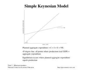
Simple Keynesian Model. Planned aggregate expenditure = C + I + G + NX 45 degree line: all points where production (real GDP) = aggregate expenditure Equilibrium occurs where planned aggregate expenditure equals production. Equilibrium and Disequilibrium in the Keynesian Model.

E N D
Simple Keynesian Model Planned aggregate expenditure = C + I + G + NX 45 degree line: all points where production (real GDP) = aggregate expenditure Equilibrium occurs where planned aggregate expenditure equals production Unit 3 : Macroeconomics National Council on Economic Education
Equilibrium and Disequilibrium in theKeynesian Model Unit 3 : Macroeconomics National Council on Economic Education
Saving and Dissaving Unit 3 : Macroeconomics National Council on Economic Education
Increase in Investment Investment increases from I to I1. Output increases from Y to Y1. Unit 3 : Macroeconomics National Council on Economic Education
Investment Demand Interest rate decreases from r to r1. Investment increases from I to I1. Unit 3 : Macroeconomics National Council on Economic Education
Different Elasticities of Investment Demand Decrease of interest rates from r to r1. With IA, investment increases from I to I2. With IB, investment increases from I to I1. IA is more elastic than IB. Unit 3 : Macroeconomics National Council on Economic Education
Aggregate Demand An increase in price from P to P1 results in a decrease in real GDP from Y to Y1 Unit 3 : Macroeconomics National Council on Economic Education
Shifts in Aggregate Demand A decrease in expected future income, in government expenditures, in the money supply or an increase in taxes will cause the AD to shift from AD to AD1. An increase in expected future income, in government expenditures or in the money supply, or a decrease in taxes will cause the AD to shift from AD to AD2. Unit 3 : Macroeconomics National Council on Economic Education
Aggregate Supply Y* represents potential real GDP. It is full-employment output. SRAS is the short-run aggregate supply curve. Unit 3 : Macroeconomics National Council on Economic Education
Aggregate Supply 1. Potential GDP increases from Y* to Y*1. The LRAS shifts to LRAS1 and the short-run aggregate supply curve shifts to SRAS1. 2. Decrease in resource prices will shift the SRAS to SRAS1. A decrease in the money wage rate does not change the LRAS. Unit 3 : Macroeconomics National Council on Economic Education
Aggregate Supply and Aggregate Demand Unit 3 : Macroeconomics National Council on Economic Education
Change in Aggregate Demand Unit 3 : Macroeconomics National Council on Economic Education
From the Short Run to the Long Run Initially the economy is at Y*, potential GDP and P. Aggregate demand increases from AD to AD1 and the economy moves to Y1 and P1. The final equilibrium is Y* and P2. Unit 3 : Macroeconomics National Council on Economic Education
Long-Run Aggregate Supply and Production Possibilities Curves Unit 3 : Macroeconomics National Council on Economic Education