Spreadsheets
Spreadsheets . Microsoft Excel. Title bar, Menu Tabs & Ribbon. Title bar – shows file name. Menu Tabs– all program functions. Cell Reference – displays active cell. Ribbon – shortcuts to program functions. Column/Row headings. Formula bar – input cell information.

Spreadsheets
E N D
Presentation Transcript
Spreadsheets Microsoft Excel
Title bar, Menu Tabs & Ribbon Title bar – shows file name Menu Tabs– all program functions Cell Reference – displays active cell Ribbon – shortcuts to program functions Column/Row headings Formula bar – input cell information Active Cell - highlighted
Enter Text or Data • Click in cell to enter data or text. Begin typing – look at formula bar for correct data entry • Click the check mark next to the formula bar or strike the enter key to accept the entry • Click the X or backspace/delete to remove the entry
Margins • Page Layout Tab > Margins drop menu • Choose pre-designed setup or Custom Margins to create your own margins • Only adjust the four major margin options - Top, Bottom, Right & Left
Header • You will put your name, assignment, class and date information in the header • Insert Tab – Header & Footer • The screen will look like it does below • Use the Tab or Ctrl+Tab to jump from left – center – right sections of the header • To return to Normal View Choose View Tab > Normal
Cell Reference • Cell Reference is the specific name of a cell. • All formulas will require the use of a cell reference – you will not just type in the number that is in a particular cell. • The first cell of a spreadsheet is A1 • Cells are named first by the column and then by the row.
Range • Group of consecutive cells • Named with two cells • First cell in the range (upper left cell) • Last cell in the range (lower right cell) The range at the right is named (B2:D6) • Ranges are surrounded by ( ) and separated by :
Format Cells • Cells must first be highlighted before formatting can take place • Cells without text can be formatted for future text use
Types of Formatting • Basic formatting • Fonts, size, B,I,U • Alignment • Font colors • Cell background colors (fill) (paint bucket on tool bar) • Data formatting (use format menu)
Data formatting in cells • Numbers and text can be formatted as general numbers, currency, percentages, decimals, dates, ect. • Highlight cell(s) to be formatted • Home Tab – Number section – Use drop menu or extend menu • If necessary, choose a decimal place
Copy/Cut & Paste • This is performed just as it is in Microsoft Word. First highlight the cell or range you would like to copy or cut. • If you are a “right click person” right click drag to copy/cut. Move mouse to new location right click paste. • If you are a “menu person” edit menu drag to copy/cut. Move mouse to new location edit paste.
Borders • Borders can be used with single cells or a range. Borders can be as simple as a line below the cells or a complete line around the cells or range. • First highlight the cell or range you would like to add the border to. • Home Tab > Borders button in font section
Insert Rows/Columns • If you need to insert a blank row or column you need to first highlight the row or column. • To highlight an entire row or column you must click on the row/column heading. • Right Click > Insert
Gridlines on working page • Borders are not gridlines. Gridlines are the lines around all of the cells you see. If you prefer to not work with gridlines as you build your spreadsheet you can turn them off using the • View Tab > Show/Hide Section > Gridlines check box • THIS IS ONLY YOUR WORKING PAGE. IT DOES NOT EFFECT YOUR PRINTED WORK.
Gridlines on Printed Page • By default, excel will not print gridlines on your spreadsheet. • To Print gridlines • Page Layout Tab > Sheet Options Section > Check box for Print Under Gridlines
Formulas • ALWAYS begin with = (equal sign) • ALWAYS use cell reference (cell name ie A3) • Formula in Cell B6 • =B4+B5
Formula options • Addition: + • Subtraction: - • Division: / • Multiplication: * Formulas in excel use order of operations =A2+(B3*B4) • B3*B4 will happen first
Show Formulas • By default excel will display formula “values” (the result of the formula). You will be asked to also show formulas and print them with each assignment. • You will lose some basic formatting and your columns will get wider. DO NOT get worked up. Ignore the loss of formatting and adjust the column widths down as needed so your spreadsheet prints on one page. • Ctrl + `(grave accent) • Switches between values and formula view
SUM Functions • Sum functions are used to ADD multiple cells in a range (3 or more cells). • Must use cell reference (ie A3) in formulas • All Formulas begin with = • Format is a follows: =SUM(A3:D3) – or whatever the range might be.
Shortcut using SUM Function • Highlight the range that contains the data to be added. • Formulas Tab > Function Library Section > Auto • Formula and answer will appear in the next cell in the range
Cell Merge • Cell Merge is used to center information over a particular range. • The title of a spreadsheet is an example • Highlight the range you want to merge over • Home Tab > Alignment Section > Merge & Center Button
Charts • Charts are a tool to quickly show the person viewing your data “what it all means.” • Once the spreadsheet is built you need to decide what you want to chart. This is to include heading. Headings help explain what the data means.
Charts cont. • Once you have decided what you need to include in your chart – highlight it • Insert Tab > Charts Section > Drop Menu for Specific Chart • Chart will embed into spreadsheet
Charts cont. • Once the chart is completed you can apply different designs and formats, you may also resize and move the chart • Double Click on the Chart to see the Chart Tools Design Tab • Expand the Charts Layout section of the design Ribbon to change the layout • Right click on different items of the chart (title, axis titles, etc) to adjust format • To delete an item (key, labels, title) click on it once and strike the delete key
Charts cont. • Each item within the chart can also be manipulated by double clicking on that individual item within the chart. • Right click – format data point