Information Retrieval System Performance Metrics and Techniques
Explore the challenges and solutions in text retrieval systems, including issues of synonymy and polysemy, the importance of word stems, and techniques like Latent Semantic Indexing. Learn about similarity measures and document retrieval methods, such as telescopic-vector trees and query executions. Discover how to assess the effectiveness of a text retrieval system using precision and recall.

Information Retrieval System Performance Metrics and Techniques
E N D
Presentation Transcript
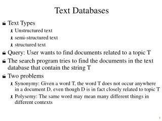
Text Databases • Text Types • Unstructured text • semi-structured text • structured text • Query: User wants to find documents related to a topic T • The search program tries to find the documents in the text database that contain the string T • Two problems • Synonymy: Given a word T, the word T does not occur anywhere in a document D, even though D is in fact closely related to topic T • Polysemy: The same word may mean many different things in different contexts
We discuss, • Measures of performance of a text retrieval system • Latent semantic indexing • Telescopic-Vector trees for document retrieval
Precision and Recall • Precision: • How many of the returned documents are relevant? • (20+1)/(20+150+1) • Recall: • How many of the relevant documents are returned? • (20+1)/(20+50+1) 50 Returned documents 20 150 Relevant documents All documents
Some Concepts • Stop List • A set of words that do not “discriminate” between the documents in a given archive • E.g.: Cornell SMART system has about 440 words on its stop list • Word Stems • Many words are small syntactic variants of each other • E.g., drug, drugged, drugs are similar in the sense that they share a common “stem,” the word drug • Most document retrieval systems first eliminate words on stop lists and reduce words to their stems, before creating a frequency table • Frequency Tables
Some Concepts • Frequency Tables • D is a set of N documents • T is a set of M words/terms occurring in the documents of D • Assume no words on the stop list for D occur in T and all words in T have been stemmed • The frequency table FreqT is an (MN) matrix such that FreqT(i,j) equals the number of occurrences of the word ti in the document dj Doc String d1 Sex, Drugs and Videotape d2 The Iranian Connection d3 Boating and Drugs: Slips owned by Cartel d4 Connections between Terrorism and Asian Dope Operations Term/Doc d1 d2 d3 d4 drug 1 0 1 0 boat 0 0 1 0 iran 0 1 0 0 connection 0 1 0 1
Similarity • d1 and d2 are similar because the distribution of the words in d1 mirrors the distribution of words in d2 • both contain lots of occurrences of t1 and t4 and relatively few occurrences of t2 and t3 and moderately many occurrences of t5 • d3 and d5 are also similar • d4 and d6 stand out as sharply different Term/Doc d1 d2 d3 d4 d5 d6 t1 615 390 10 10 18 65 t2 15 4 76 217 91 816 t3 2 8 815 142 765 1 t4 312 511 677 11 711 2 t5 45 33 516 64 491 59
Similarity • Is merely counting words enough? • It does not indicate the importance of the words • What about document lengths? • We should also include the importance of the word in the document - How? • If a word occurs 3 times in a 100 word document may have more significance than if it occurs 3 times in a million word document • ratio of the number of occurrences of a word to the total number of words
Queries • User wants to execute the query • Find the 25 documents that are maximally relevant wrt banking operations and drugs? • After stemming, relevant keywords are “drug, bank” • Assume the query Q as vector • We want to find the columns in FreqT that are as close as possible to the Q’s vector • Closeness Metrics • Term Distance: (between Q and dr) = Mj = 1 (vecQ(j) - FreqT(j,r))2 • Cosine Distance: Mj = 1 (vecQ(j) FreqT(j,r)) Mj = 1 (vecQ(j))2 Mj = 1 (FreqT(j,r))2 • Complexity of retrievals may be O(NM) which could be very large (Latent Semantic Indexing- A solution!!!)
Latent Semantic Indexing • The number of documents M and the number of terms N is very large • N could be over 10,000,000 (English words, proper nouns) • LSI tries to find a relatively small subset of K words which discriminate between M documents in the archive • LSI is claimed to work effectively for around K = 200 • Advantage: Each document is now a column vector of length 200, instead of length N (This is a big plus!!!) • But, how do we find such a subset K? • A technique called singular valued decomposition
LSI • 4 steps approach used by LSI • Table creation: Creation of the frequency matrix FreqT • SVD Construction: Compute the singular valued decompositions (A,S,B) of FreqT • Vector Identification: For each document d, let vec(d) be the set of all terms in FreqT whose corresponding rows have not been eliminated in the singular matrix S • Index Creation: Store the set of all vec(d)’s indexed by any one of the number of techniques (such as TV-tree)
Singular Valued Decomposition • Let M1 and M2 are two matrices of order (m1n1) and (m2n2), respectively • M1 M2 is well defined iff n1 = m2 • Transpose of M, MT • Vector = matrix of order (1m) 3 2 1 4 3 7 20 21 = 4 8 2 4 6 20 48 60 T 7 20 21 7 20 20 48 60 = 20 48 21 60
Singular Valued Decomposition • Two vectors X and Y of the same order are said to be orthogonal iff XTY = 0 • X = [10, 5, 20], Y = [1, 2, -1] • A Matrix M is orthogonal iff MTM is the identity matrix 10 0 XTY = 5 [1 2 -1] = 0 20 0 1 1 M = is orthogonal 0 0
Singular Valued Decomposition • Matrix Mis said to be diagonal iff the order of M is (mm) and for all 1 i, j m, i j M(i,j) = 0 • A and B are diagonal, but C is not • A diagonal matrix M of order (mm) is said to be non-decreasing iff for all 1 i, j m, i j M(i,i) M(j,j) • A is a non-decreasing diagonal matrix but B is not 1 0 0 1 0 0 1 1 A = 0 4 0 ; B = 0 0 0 ; C = 0 0 5 0 0 0 0 0
SVD • A singular value decomposition of FreqT is a triple (A,S,B) where: • 1. FreqT = (ASBT) • 2. A is an (M M) orthogonal matrix such that ATA = I • 3. B is an (N N) orthogonal matrix such that BTB = I • 4. S is a diagonal matrix called a singular matrix • Theorem: Given any matrix M of order (m m), it is possible to find a singular value decomposition, (A,S,B) of M such that S is a non-decreasing diagonal matrix • The SVD of the matrix 1.44 0.52 is given by: 0.92 1.44 .6 -.8 5 0 .8 .6 here the singular values are 5,2 .8 .6 0 2 .6 -.8 and the singular matrix S is non-decreasing
Returning to LSI • Given a frequency matrix FreqT, we can decompose it into SVD TSDT where S is non-decreasing • If FreqT is of size (M N), then T is of size (M M) and S is of order (M R) where R is the rank of FreqT, and DT is of the order (R N) • We can now shrink the problem substantially by eliminating the least significant singular values from the singular matrix S • Choose an integer k that is substantially smaller than R • Replace S by S*, which is a (k k) matrix such that S*(i,j) = S(i,j) for 1 i, j k • Replace the (R N) matrix DT by the (k N) matrix D*T where D*T(i,j) = DT(i,j) if 1 i k and 1 j N
LSI • How? • Bottom line: • Throw away the least significant values and retain the rest of the matrix • Key claim in LSI is that if k is chosen judiciously, then the k rows appearing in the singular matrix S* represent the k “most important” (from the point of view of retrieval) terms occurring in the “entire” document 20 0 0 0 0 0 16 0 0 0 0 0 12 0 0 0 0 .08 0 0 0 0 0 .004 20 0 0 0 16 0 0 0 12
Analysis • Usually R is taken to be 200 • The size of FreqT is (M N), • where M = number of terms = 1,000,000 • N = number of documents = 10,000 (even for a small database) • After shrinking the singular matrix to 200 • the first matrix: (M R) = 1,000,000 200 = 200,000,000 • the singular matrix: (R R) = 200 200 = 400,000 (only 200 need to be stored because all others are 0’s) • the last matrix: (R N) = 200 10,000 • A total of 202,000,200 (200 million) • In contrast, (M N) is close to 10,000 million!!! • SVD reduced the space utilized to about 1/50th of that required by the original frequency table
LSI: Document Retrieval using SVD • Given 2 documents d1 and d2 in the archive, how similar are they? • Given a query string/document Q, what are the n documents in the archive that are most relevant for the query? • Dot Product • Suppose x = (x1, … xw) and y = (y1, …, yw) • The dot product of x and y = x y = xi yi (where i = 1,..w) • Similarity of these two documents wrt the SVD representation TS*D*T of a freq table is the dot product of the two columns in the matrix D*T of the two documents
LSI: Document Retrieval using SVD • The top p matches for Q • 1. For all 1 i j p, the similarity between vecQ and di is greater than or equal to the similarity between vecQ and dj • 2. There is no other document dz such that the similarity between dz and vecQ exceeds that of dp • Can be done by using any indexing structure for R-dimensional spaces (R-trees, k-d trees) • However R-trees, k-d trees do not work well for high-dimensional data (>20) • Solution: TV-trees!
Telescopic Vector (TV) Trees • Access to point data in very large dimensional spaces should be highly efficient • A document d may be viewed as a vector v of length k, where the singular matrix is of size (k k) • Thus each document is a point in a k-dimensional space • A document database is a collection of such points • To find the top p matches for Q, expressed as vecQ of length k, we need to find the k-nearest neighbors vecQ • TV-tree isa data structure similar to R-trees
Organization of a TV-tree • NumChild: Max number of a node is allowed to have • : is a number, > 0, < k is the number of active dimensions • Each in TV(k,NumChild,) represents a region, for this purpose, each node contains 3 fields • N.Center: this is a point in k-dimensional space • N.Radius: A real number > 0 • N.ActiveDims: A list of at most dimensions, It is a subset of {1,…k} of cardinality or less
Region associated with a node N • Suppose x and y are points in k-dim space • act-dist(x,y) = (xi- yi)2 where i ActiveDims • Let k = 200, = 5 and the set of ActiveDims = {1,2,3,4,5} • x = (10,5,11,13,7,x6, ….x200) • y = (2,4,14,8,6,y6, …y200) • act-dist(x,y) = (10-2)2 + (5-4)2 + (11-14)2 + (13-8)2 + (7-6)2 = 10 • Node N represents the region containing all points x such that the active distance between x and N.Center N.Radius • if N.Center = (10,5,11,13,7,0,0,0…0) • N.ActiveDims = {1,2,3,4,5} • then N represents the region consisting of all points x such that (x1-10)2 + (x2-5)2 + (x3-14)2 + (x4-13)2 + (x5-7)2 N.Radius • A node also contains an array, Child, of pointers to other nodes
Properties of TV- Trees • All data is stored at the leaf nodes • Each node (except the root and the leaves) must be at least half full • If N is a node, and N1, .. Nr are its children, then • Region(N) is Union of all Region(Ni)’s
Insertion into TV-trees • Three steps: • 1. Branch Selection: When we insert a new vector v at node N, • for each child Nj of N, compute exp(v) = the amount we must expand Nj.Radius so that v’s active distance from Nj.Center falls within this region • select a branch such that exp(v) is minimum • 2. Splitting: When a leaf node is full and cannot accommodate the new vector v, we have to split. • Split vectors into 2 groups G1,H1 such that we enclose all vectors in G1 with center c1 and radius r1, and all in H1 with center c1’ and r1’ • There exist many such cases: G2,H2 (with (c2,r2), (c2’,r2’) • take the one with minimum sum of radii, i.e., G1,H1 is better if (r1+r1’) < (r2+r2’)
Insertion into TV-trees • 3. Telescoping: The active dimensions associated with a node or the children of the node change (either expand or contract); this is called telescoping. This happens in 2 cases: • When a node splits into two subnodes N1 and N2, vectors in region(N1) all agree on not just the active dimensions of N, but a few more as well • When a new vector is added to a node N, the active dimensions may reduce
Other Retrieval Techniques: Inverted Indices • A document_record contains 2 fields: doc_id, postings_list • postings_list is a list of terms (or pointers to terms) that occur in the document. Sorted using a suitable relevance measure • A term_record consists of 2 fields: term, postings_list • postings_list is list specifying which documents the term appeared in • Two hash tables are maintained: DocTable, TermTable • DocTable is constructed by hashing on doc_id • TermTable by hashing on term • To find all documents associated with a term, merely return the postings_list
Other Retrieval Techniques: Signature Files • Associate a signature with each document • signature: is a representation of an ordered list of terms that describe the document • the list of terms in the signature may be derived from a frequency analysis, stemming, usage of stop lists