B asic L ocal A lignment S earch T ool
B asic L ocal A lignment S earch T ool. Presented by Mei Liu August 7, 2008. Introduction. BLAST Finds regions of local similarity between sequences Assesses which DNA or protein sequences in a large database have significant similarity with a given query sequence


B asic L ocal A lignment S earch T ool
E N D
Presentation Transcript
Basic Local Alignment Search Tool Presented by Mei Liu August 7, 2008
Introduction • BLAST • Finds regions of local similarity between sequences • Assesses which DNA or protein sequences in a large database have significant similarity with a given query sequence • Infer functional and evolutionary relationships between sequences • Help identify members of gene families • Two implementations of BLAST: one by NCBI and the other at Washington University
Introduction • WU-BLAST printouts give the following values • Score or High Score • Bit scores • Expect values • P-values
Outline • Comparison of two aligned sequences • BLAST random walk • Parameter calculations • Choice of score • Bounds and approximation for BLAST p-value • Normalized and bit scores • Number of high-scoring excursions • Karlin-Altschul sum statistic
Outline • Comparison of two unaligned sequences • Comparison of a query sequence against a database • Minimum significance lengths • Parametric or non-parametric test? • Gapped BLAST and PSI BLAST
1. Two Aligned Sequences • Given an ungapped global alignment of two protein sequences, both of length N • Null hypothesis: for each aligned pair of amino acids, the two amino acids are generated by independent mechanisms • Null hypothesis probability of the amino acid pair (j, k) = • Alternative hypothesis probability of the amino acid pair (j, k) = (10.1) (10.2)
1.1 BLAST Random Walk • Number the positions from left to right as 1, 2, …, N • A score S(j, k) is allocated to each aligned amino acid pair (j, k) • In application of BLAST, the score is found by BLOSUM or PAM
1.1 BLAST Random Walk • PAM • Developed by Margaret Dayhoff in 1970s • calculated by observing the differences in closely related proteins • PAM1 matrix estimates what rate of substitution would be expected if 1% of the amino acids had changed • Derived matrices as high as PAM250 • Higher numbers in the PAM matrix naming scheme denote larger evolutionary distance • Not work very well for aligning evolutionarily divergent sequences
1.1 BLAST Random Walk • BLOSUM • Henikoff and Henikoff constructed these matrices using multiple alignments of evolutionarily divergent proteins • Probabilities used in the matrix calculation are computed by looking at "blocks" of conserved sequences found in multiple protein alignments • To reduce bias from closely related sequences, segments in a block with a sequence identity above a certain threshold were clustered • For the BLOSUM62, this threshold was set at 62% • Larger numbers in the BLOSUM matrix naming scheme denote higher sequence similarity
1.1 BLAST Random Walk • Accumulated score at position i is calculated as the sum of scores for various amino acid comparisons at positions 1, 2, … , i Sequence 1: T Q L A A W C R M T C F E I E C K V Sequence 2: R H L D S W R R A S D D A R I E E G S(j, k): -1, 1, 5, -2, 1, 15, -4, 7, -1, 2, -4, etc. Accumulated Score: -1, 0, 5, 3, 4, 19, 15, 22, etc.
1.1 BLAST Random Walk • Let Y1, Y2, … be the respective maximum heights of the walk relative to the height of any ladder point after leaving this ladder point and before arriving at the next • Define Ymax as the maximum of these maxima • Ymax is the test statistic used in BLAST, so it is necessary to find its null hypothesis distribution • Random variables Yi exhibit geometric-like distribution • C and depends on the substitution matrix used and amino acid frequencies { } and { } • Probability distribution of Ymax, apart from C and , also depends on the mean number of ladder points in the walk
1.2 Parameter Calculations • Step size is identified with a score S(j,k) • Null hypothesis probability of taking a step of any size is found from the two sets of frequencies { } and { } • When null hypothesis is true, can be calculated (7.61) (10.3)
1.2 Parameter Calculations • Ymax depends on C, , and mean number of ladder points in BLAST walk • Mean number of ladder points in turn depends on the distance A between ladder points • Calculation of A depends on the calculation of R-j • Two alternative approaches in calculation (7.41)
1.2 Parameter Calculations • Decomposition of paths • Ex. A walk with 2 possible steps: +1, -2 with respective probabilities p, q=1-p • Any ladder point reached in the walk is at a distance 1 or 2 below the previous one • Respective probabilities of the two cases are R-1 and R-2 = 1 – R-1 • Probability that -2 is a ladder point is: • Probability that it goes to -2 immediately, and • Probability that it first goes to +1 reaches 0 -2
1.2 Parameter Calculations (10.4) Directly -2 +1 0 -2 (10.5) • Then value of A follows from Eq. (7.41) • Since two sequences compared are each of length N, and mean distance between ladder points is A • The mean number of ladder points is N/A (7.41)
1.3 Choice of a Score • BLAST score is a log likelihood ratio • Why? • Similar to sequence analysis • If random variable Y has a discrete probability distribution, this “score” statistic is defined as the log likelihood ratio • If amino acid pair (j,k) is observed at any position, and if pjpk' and q(j,k) are null and alternative hypothesis probabilities (10.6)
1.3 Choice of a Score • Second argument leads to the choice of a specific proportionality constant • Suppose some arbitrary substitution matrix is chosen with (j,k) element S(j,k), let q(j,k) be defined implicitly by • where is defined in equation (10.3) • Thus q(j,k) can be defined explicitly by (10.7) (10.3) (10.8)
1.3 Choice of a Score • Karlin and Altschul (1990) and Karlin (1994) showed that • When null hypothesis is true, the frequency with which the observation (j,k) arises in high-scoring excursions is asymptotically equal to q(j,k) • Then argued that a score scheme is “optimal” if the frequency of the observation (j,k) in high-scoring excursions is asymptotically equal to the “target” frequency q(j,k), the frequency arising if the alternative hypothesis is true • i.e. frequency in the most biologically relevant alignments of conserved regions
1.3 Choice of a Score • Argument for the use of S(j,k) as the score statistic lead to following procedures: • Various possibilities for q(j,k) • One frequently adopted choice is derived from the evolutionary arguments that lead to PAMn matrix construction in 6.5.3 (10.7) (10.9) (10.10)
1.3 Choice of a Score • Choice of S(j,k) can as be related to relative entropy • Score defined is proportional to the support given by the observation (j,k) in favor of the alternative hypothesis over the null hypothesis • Eq. 1.124 shows that when the alternative hypothesis is true, the mean support for the alternative over the null hypothesis is (10.7) (10.11) (10.12)
1.3 Choice of a Score • Mean score in high-scoring segments is asymptotically (10.7) (10.12) (10.13)
1.3 Choice of a Score • Simulations show that the convergence to this asymptotic value is very slow • Direct computation of H is not possible • and S(j,k) are known, but q(j,k) is unknown • BLAST uses indirect approach to calculate H where q(j,k) is first calculated by (10.12) (10.8)
1.4 Bounds and Approximation for BLAST P-value • Test statistic used in BLAST is the maximum Ymax of • n ≈ N/A random variables • Each being a random upwards excursion height following a ladder point in the BLAST random walk • In section 7.6.4, it was shown that each upward excursion has the geometric-like distribution • Obtain asymptotic bounds for the null hypothesis distribution of Ymax and hence asymptotic bounds for a BLAST P-value
1.4 Bounds and Approximation for BLAST P-value • There exists an asymptotic distribution for the maximum of n iid continuous random variables whose density function has support of the form (A, +∞) • However, Ymax is a discrete random variable • Use the continuous distribution results to find asymptotic bounds for the distribution of Ymax • If Xmax is the max of n iid continuous r.v. and if Ymax = floor(Xmax), then Ymax is a discrete r.v. • Thus, for any positive integer y (10.14)
1.4 Bounds and Approximation for BLAST P-value • Let Xmax be the max of n iid r.v. each having exponential distribution and Ymax = Floor(Xmax) • Ymax has the same distribution as the max of n iid r.v. each having geometric distribution • Applying Eq. (2.130) and bounds in (10.14), we have a close approximation (10.15) (10.16) (10.17)
1.4 Bounds and Approximation for BLAST P-value • If we replace n by N/A for the mean number of BLAST ladder points and define a new parameter K by • The inequality (10.17) becomes • If replace y by x+-1logN, we have (10.18) (10.19) (10.20) (10.21) (10.22)
1.4 Bounds and Approximation for BLAST P-value • These bounds for BLAST P-value are not directly relevant in practice because • BLAST search involves comparison of short query sequence with a large DB with many fragments • No a priori alignment • Nevertheless, P-value approximation derives ultimately from the lower P-value bound in Eq. (10.22) • More appropriate to use conservative (overestimate the true P-value) upper bound in (10.22) rather than lower bound
1.5 Normalized and Bit Scores • Karlin and Altschul (1993) call the following expression a “normalized score” • In terms of this score, the inequalities (10.20) can be written as • From the upper inequality • P-value corresponding to an observed value s' is (10.25) (10.26) (10.27) (10.28)
1.5 Normalized and Bit Scores • BLAST record a score similar to the normalized score S', namely the “bit” score defined by
1.6 Number of High-Scoring Excursions • Quantity E' = quantity “Expect” in BLAST • Under null hypothesis, for each excursion, the maximum height Y has a geometric-like distribution • # of excursions = N/A • In BLAST, mean number of excursions reaching a height v or more is approximately (10.18) (10.34)
1.6 Number of High-Scoring Excursions • Expected value of the number of excursions corresponding to the observed maximal score ymax (10.35) (10.36) (10.37)
1.7 Karlin-Altschul Sum Statistic • Focusing on Ymax loses information provided by heights of the 2nd, 3rd, etc. excursions in the random walk • Consider r largest Yi values • Compute r normalized scores where (10.38)
1.7 Karlin-Altschul Sum Statistic • Karlin and Altschul (1993) showed that to a close approximation, the null hypothesis joint density function is • Any reasonable function of can be the test statistic • Use transformation methods introduced in Chap. 2 to find the distribution of this test statistic • In turn allows computations of P-value and E or Expect value corresponding to any observed value of this statistic (10.39)
1.7 Karlin-Altschul Sum Statistic • Statistic suggested is the sum of the normalized scores, called the Karlin-Altschul sum statistic • Null hypothesis density function f(t) of Tr • When t is sufficiently large, this density function can be used to find the approximate expression (10.40) (10.41)
1.7 Karlin-Altschul Sum Statistic • The approximation (10.41) is sufficiently accurate when t > r(r+1), and BLAST uses it when the inequality holds • If t is the observed value of Tr, the right hand side in (10.41) provides the approximate P-value corresponding to this observed value • This is used as a component of the eventual BLAST printout P-value • Ex. s1 = 4.4 and s2 = 2.5 • r = 1, P-value for the highest normalized score 4.4 = e-4.4 = 0.012 • r = 2, P-value for the sum 6.9 = 6.9/2 * e-6.9 = 0.0035 (10.41)
2. Two Unaligned Sequences • Given two sequences of lengths N1 and N2, but no specific alignment is given • Need to find the significance of high-scoring segment pairs between all possible (ungapped) local alignments
2.1 Theoretical and Empirical Background • BLAST considers all ungapped alignments determined by all possible relative positions of two sequences • For each relative position, alignment is extended as far as possible in either direction, giving a total of N1+N2-1 ungapped alignments
2.1 Theoretical and Empirical Background • Each alignment yields a random walk • Total N1N2 comparisons between two sequences taking all possible positions relative to each other • Many conclusions from previous section can be carried over to the present case • with N replaced by N1N2 • or a more refined function allowing for edge effects
2.1 Theoretical and Empirical Background • Ymax is the maximum score achieved in the random walk comparing sequences, using all possible ungapped local alignments • Mean number of ladder points: • Assume null hypothesis is true, inequalities in (10.21) is replaced by • Normalized score S' is redefined as • Expected number E' of excursions reaching a height ymax or more is • Null hypothesis mean of Ymax is (10.42) (10.43) (10.44) (10.45) (10.46)
2.2 Edge Effects • A high-scoring random walk excursion might be cut short at the end of a sequence match • So the height of high-scoring excursions and the number of such excursions will be less than predicted by theory • Edge effects is an important factor in the comparison of two comparatively short sequences • BLAST theory concerns two long sequences • In practice, BLAST considers databases of large number of short sequences
2.2 Edge Effects • BLAST calculations allow for edge effects by subtracting from both N1 and N2 a factor depending on the mean length of any high-scoring excursion • Eq. (10.13) showed that the mean value of the step in high-scoring excursion asymptotically approaches • Given the height achieved by a high-scoring excursion is denoted by y, the mean length E(L|y) of this excursion, conditional on y, is • BLAST theory replaces N1 and N2 by (10.47)
2.2 Edge Effects • Specifically, the normalized score is replaced by • Expected number of excursions scoring v or higher is replaced by • E' is given by (10.48) (10.49) (10.50) (10.51)
2.2 Edge Effects • The use of edge correction in (10.49) assumes that asymptotic formula for the mean step size in a high-scoring excursion is appropriate • Values calculated from Eq. (10.47) is inaccurate for anything other than very large values of N • Use of edge correction in (10.49) might in practice lead to P-value estimates less than the correct values for anything other than very large N (10.47)
2.2 Edge Effects • In BLAST, edge effect correction factor for the Karlin-Altschul sum statistic Tr is calculated as follows • Raw edge effect correction is calculated as • Edge correction value E(L) is defined by • f is an “overlap adjustment factor” that can be chosen by the user • Default f = 0.125 implies that overlaps between segments of up to 12.5% are allowed (10.52)
2.3 Multiple Testing • No obvious choice for the value of r • BLAST considers all r = 1, 2, 3, … and choose the set of HSPs with lowest sum statistic P-value as the most significant • However, it implies that a sequence of tests, one for each r • So issue of multiple testing arises • Ignoring multiple testing issue can lead to a significant overestimate of BLAST P-values • Unfortunately, no rigorous theory available to deal with this issue • In practice, it is handled in an ad hoc manner
2.3 Multiple Testing • Ex. WU-BLAST • P-value is adjusted by dividing by a factor • When r = 1, the factor became 1- π, which implies that E' is divided by 1- π • BLAST default value 0.5 of π implies that E=2E', so that • P-value is then found as (10.56) (10.57)
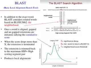
3. Query Sequence vs. Database • Compare query sequence to each database sequence to obtain P-values for individual comparisons • For r = 1, probability that in a match with score v or more is • Expect, the mean number of HSPs scoring v or more in the entire database is given by • D = total length of DB (sum of lengths of all database sequences) • N2 = length of the database sequence (10.58) (10.59) (10.60)