Download

1 / 24
240 likes | 264 Views
Dive into the world of Markov processes and Hidden Markov Models (HMMs) with a comprehensive overview of their applications, assumptions, and computations. Explore how these models are used in scenarios like weather prediction and speech recognition, and understand their limitations and workarounds.

E N D
Instructor: Vincent Conitzer CPS 570: Artificial IntelligenceMarkov processes and Hidden Markov Models (HMMs)
Motivation • The Bayes nets we considered so far were static: they referred to a single point in time • E.g., medical diagnosis • Agent needs to model how the world evolves • Speech recognition software needs to process speech over time • Artificially intelligent software assistant needs to keep track of user’s intentions over time • … … …
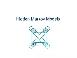
Markov processes • We have time periods t = 0, 1, 2, … • In each period t, the world is in a certain state St • The Markov assumption: given St, St+1 is independent of all Si with i < t • P(St+1 | S1, S2, …, St) = P(St+1 | St) • Given the current state, history tells us nothing more about the future S3 St S1 S2 … … • Typically, all the CPTs are the same: • For all t, P(St+1 = j | St = i) = aij (stationarity assumption)
Weather example • St is one of {s, c, r} (sun, cloudy, rain) • Transition probabilities: .6 s .1 .3 .4 not a Bayes net! .3 .2 c r .3 .3 .5 • Also need to specify an initial distribution P(S0) • Throughout, assume P(S0 = s) = 1
Weather example… .6 s .1 .3 .4 .3 .2 c r .3 .3 .5 • What is the probability that it rains two days from now? P(S2 = r) • P(S2 = r) = P(S2 = r, S1 = r) + P(S2 = r, S1 = s) + P(S2 = r, S1 = c) = .1*.3 + .6*.1 + .3*.3 = .18
Weather example… .6 s .1 .3 .4 .3 .2 c r .3 .3 .5 • What is the probability that it rains three days from now? • Computationally inefficient way: P(S3 = r) = P(S3 = r, S2 = r, S1 = r) + P(S3 = r, S2 = r, S1 = s) + … • For n periods into the future, need to sum over 3n-1 paths
Weather example… .6 s .1 .3 .4 .3 .2 c r .3 .3 .5 • More efficient: • P(S3 = r) = P(S3 = r, S2 = r) + P(S3 = r, S2 = s) + P(S3 = r, S2 = c) = P(S3 = r | S2 = r)P(S2 = r) + P(S3 = r | S2 = s)P(S2 = s) + P(S3 = r | S2 = c)P(S2 = c) • Only hard part: figure out P(S2) • Main idea: compute distribution P(S1), then P(S2), then P(S3) • Linear in number of periods! example on board
Stationary distributions • As t goes to infinity, “generally,” the distribution P(St) will converge to a stationary distribution • A distribution given by probabilitiesπi (where i is a state) is stationary if: P(St = i) =πi means that P(St+1 = i) =πi • Of course, P(St+1 = i) = ΣjP(St+1 = i, St = j) = ΣjP(St = j) aji • So, stationary distribution is defined by πi = Σj πj aji
Computing the stationary distribution .6 s .1 • πs = .6πs + .4πc + .2πr • πc = .3πs + .3πc + .5πr • πr = .1πs + .3πc + .3πr .3 .4 .3 .2 c r .3 .3 .5
Restrictiveness of Markov models • Are past and future really independent given current state? • E.g., suppose that when it rains, it rains for at most 2 days S3 S4 S1 S2 … • Second-order Markov process • Workaround: change meaning of “state” to events of last 2 days … S3, S4 S4, S5 S2, S3 S1, S2 • Another approach: add more information to the state • E.g., the full state of the world would include whether the sky is full of water • Additional information may not be observable • Blowup of number of states…
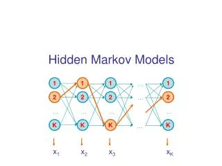
Hidden Markov models (HMMs) • Same as Markov model, except we cannot see the state • Instead, we only see an observation each period, which depends on the current state S3 St S1 S2 … … O3 Ot O1 O2 … … • Still need a transition model: P(St+1 = j | St = i) = aij • Also need an observation model: P(Ot = k | St = i) = bik
Weather example extended to HMM • Transition probabilities: .6 s .1 .3 .4 .3 .2 c r .3 .3 .5 • Observation: labmate wet or dry • bsw = .1, bcw = .3, brw = .8
HMM weather example: a question .6 bsw = .1 bcw = .3 brw = .8 s .1 .3 .4 .3 .2 c r .3 .3 .5 • You have been stuck in the lab for three days (!) • On those days, your labmate was dry, wet, wet, respectively • What is the probability that it is now raining outside? • P(S2 = r | O0 = d, O1 = w, O2 = w) • By Bayes’ rule, really want to know P(S2, O0 = d, O1 = w, O2 = w)
Solving the question .6 bsw = .1 bcw = .3 brw = .8 s .1 .3 .4 .3 .2 c r .3 .3 .5 • Computationally efficient approach: first compute • P(S1 = i, O0 = d, O1 = w) for all states i • General case: solve for P(St, O0 = o0,O1 = o1, …,Ot = ot) for t=1, then t=2, … This is called monitoring • P(St, O0 = o0,O1 = o1, …,Ot = ot) = Σst-1 P(St-1 = st-1, O0 = o0,O1 = o1, …,Ot-1 = ot-1) P(St | St-1 = st-1) P(Ot = ot | St)
Predicting further out .6 bsw = .1 bcw = .3 brw = .8 s .1 .3 .4 .3 .2 c r .3 .3 .5 • You have been stuck in the lab for three days • On those days, your labmate was dry, wet, wet, respectively • What is the probability that two days from now it will be raining outside? • P(S4 = r | O0 = d, O1 = w, O2 = w)
Predicting further out, continued… .6 bsw = .1 bcw = .3 brw = .8 s .1 .3 .4 .3 .2 c r .3 .3 .5 • Want to know: P(S4 = r | O0 = d, O1 = w, O2 = w) • Already know how to get: P(S2 | O0 = d, O1 = w, O2 = w) • P(S3 = r | O0 = d, O1 = w, O2 = w) = • Σs2P(S3 = r, S2 = s2 | O0 = d, O1 = w, O2 = w) • Σs2P(S3 = r | S2 = s2)P(S2 = s2 | O0 = d, O1 = w, O2 = w) • Etc. for S4 • So: monitoring first, then straightforward Markov process updates
Integrating newer information .6 bsw = .1 bcw = .3 brw = .8 s .1 .3 .4 .3 .2 c r .3 .3 .5 • You have been stuck in the lab for four days (!) • On those days, your labmate was dry, wet, wet, dry respectively • What is the probability that two days ago it was raining outside? P(S1 = r | O0 = d, O1 = w, O2 = w, O3 = d) • Smoothing or hindsight problem
Hindsight problem continued… .6 bsw = .1 bcw = .3 brw = .8 s .1 .3 .4 .3 .2 c r .3 .3 .5 • Want: P(S1 = r | O0 = d, O1 = w, O2 = w, O3 = d) • “Partial” application of Bayes’ rule: • P(S1 = r | O0 = d, O1 = w, O2 = w, O3 = d) = • P(S1 = r, O2 = w, O3 = d | O0 = d, O1 = w) / • P(O2 = w, O3 = d | O0 = d, O1 = w) • So really want to know P(S1, O2 = w, O3 = d | O0 = d, O1 = w)
Hindsight problem continued… .6 bsw = .1 bcw = .3 brw = .8 s .1 .3 .4 .3 .2 c r .3 .3 .5 • Want to know P(S1 = r, O2 = w, O3 = d | O0 = d, O1 = w) • P(S1 = r, O2 = w, O3 = d | O0 = d, O1 = w) = • P(S1 = r | O0 = d, O1 = w) P(O2 = w, O3 = d | S1 = r) • Already know how to compute P(S1 = r | O0 = d, O1 = w) • Just need to compute P(O2 = w, O3 = d | S1 = r)
Hindsight problem continued… .6 bsw = .1 bcw = .3 brw = .8 s .1 .3 .4 .3 .2 c r .3 .3 .5 • Just need to compute P(O2 = w, O3 = d | S1 = r) • P(O2 = w, O3 = d | S1 = r) = • Σs2P(S2 = s2, O2 = w, O3 = d | S1 = r) = • Σs2P(S2 = s2 | S1 = r) P(O2 = w | S2 = s2) P(O3 = d | S2 = s2) • First two factors directly in the model; last factor is a “smaller” problem of the same kind • Use dynamic programming, backwards from the future • Similar to forwards approach from the past
Backwards reasoning in general • Want to know P(Ok+1 = ok+1, …, Ot = ot | Sk) • First compute • P(Ot = ot | St-1) =Σst P(St = st | St-1)P(Ot = ot | St = st) • Then compute • P(Ot = ot, Ot-1 = ot-1 | St-2) =Σst-1 P(St-1 = st-1 | St-2)P(Ot-1 = ot-1 | St-1 = st-1) P(Ot = ot | St-1 = st-1) • Etc.
Variable elimination • Because all of this is inference in a Bayes net, we can also just do variable elimination S3 St S1 S2 … … O3 Ot O1 O2 … … • E.g., P(S3 = r, O1 = d, O2 = w, O3 = w) = Σs2Σs1 P(S1=s1)P(O1=d|S1=s1)P(S2=s2|S1=s1) P(O2=w|S2=s2)P(S3=r|S2=s2)P(O3=w|S3=r) • It’s a tree, so variable elimination works well
Dynamic Bayes Nets • So far assumed that each period has one variable for state, one variable for observation • Often better to divide state and observation up into multiple variables weather in Durham, 1 weather in Durham, 2 … NC wind, 1 NC wind, 2 weather in Beaufort, 1 weather in Beaufort, 2 edges both within a period, and from one period to the next…
Some interesting things we skipped • Finding the most likely sequence of states, given observations • Not necessary equal to the sequence of most likely states! (example?) • Viterbi algorithm • Key idea: for each period t, for every state, keep track of most likely sequence to that state at that period, given evidence up to that period • Continuous variables • Approximate inference methods • Particle filtering