Download
1 / 35
370 likes | 417 Views
Explore the history of Earth's climate, from the rise of atmospheric O2 to the phenomenon of Snowball Earth ice ages. Discover possible triggers, models, and recovery processes, shedding light on how life endured during extreme glaciations.

E N D
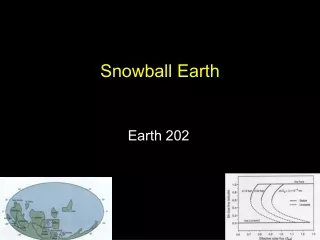
Snowball Earth Earth 202
Before talking about Snowball Earth, let’s look briefly at Earth’s long-term climate history
Ice age (Pleistocene) Dinosaurs go extinct Phanerozoic Time First dinosaurs Ice age First vascular plants on land Ice age Age of fish First shelly fossils
Geologic time First shelly fossils (Cambrian explosion) Snowball Earth ice ages Warm Rise of atmospheric O2(Ice age) Ice age Warm (?)
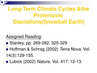
Low Latitude Glaciations • Paleomagnetic data indicate low-latitude glaciation at 2.3 Ga, 0.75 Ga, and 0.6 Ga • Paleoproterozoic glaciations (~2.3 Ga) may be triggered by the rise of O2 and the corresponding loss of CH4 • Late Precambrian glaciations studied by Hoffman et al., Science 281, 1342 (1998)
The Great Infra-Cambrian Ice AgeW. Brian Harland & M.J.S. Rudwick, Scientific American 211 (2), 28-36, 1964 Courtesy of Joe Kirschvink
Using Magnetic Data to Determine Paleolatitudes Polar Equatorial Courtesy of Adam Maloof
Periglacial Outwash Varves From the Elatina Formation, South Australia Courtesy of Joe Kirschvink
Late Precambrian Geography*(according to Scotese) * glacial deposits Hyde et al., Nature, 2000
Possible Explanations for Low-Latitude Glaciation • High obliquity hypothesis (George Williams, papers since1970’s) • Equatorial glaciation predicted for obliquities exceeding 54o • Explains how the photosynthetic algae and other life forms survived (polar regions remain ice-free) • Difficult to explain dynamically • Inconsistent with evidence (just shown) for high-latitude glaciation
Possible Explanations for Low-Latitude Glaciation (cont.) 2.“Slushball Earth” model (Hyde et al., Nature, 2000) • Tropics remain ice-free (+25o to 25o latitude) photosynthetic algae survive • Climate state is metastable and, hence, improbable • Requires large mountain ranges on paleo-Australia that do not appear to have existed • Has difficulty explaining cap carbonates…
Ghaub Glaciation(Namibia) Maieberg “cap” Glacial tillite Courtesy of Joe Kirshvink
Possible explanations for low-latitude glaciation (cont.) • “Snowball Earth” model (Joe Kirshvink, 1990) • Easy to explain from a climatic standpoint • Accounts for cap carbonates (indeed, it predicts them!) • Accounts for reappearance of BIFs • “Hard Snowball” model (km-thick ice everywhere) poses significant problems for the photosynthetic biota
Triggering a Snowball Earth • Need to get CO2 levels below ~2.5 PAL at 600 Ma, for S/S0 = 0.95 (Hyde et al.) • Possible ways to do this • Continental rifting created new shelf area, thereby promoting burial of organic carbon (Hoffman et al., Science, 1998) • Clustering of continents at low latitudes allows silicate weathering to proceed even as the global climate gets cold (Marshall et al., JGR, 1988) • Various triggers involving CH4
In any case, ice albedo feedbacktakes over when the polar caps reach some critical latitude (near 30o)
Increasing CO2 Modern Earth Caldeira and Kasting, Nature (1992)
Recovering from a Snowball Earth episode • Volcanic CO2 builds up to ~0.1 bar over a time span of ~30 m.y. (old result—Caldeira and Kasting) • This estimate may be too low (Pierrehumbert, Nature, 2004) • Our “thin-ice” model recovers at much lower CO2 levels, which it reaches more quickly
The carbonate-silicate cycle (metamorphism) • Silicate weathering slows down as the Earth cools • atmospheric CO2 should build up
Recovering from a Snowball Earth episode • Once the meltback begins, the ice melts catastrophically (within a few thousand years) • Surface temperatures climb briefly to 50-60oC • Post-Snowball temperatures would be 10-15o lower in the thin-ice model • CO2 is rapidly removed by silicate (and carbonate) weathering, forming cap carbonates
How did photosynthetic life survive the Snowball Earth? • Refugia such as Iceland? • Tidal cracks, meltwater ponds, tropical polynyas? (Hoffman and Schrag, Terra Nova, 2002) • “Thin ice” model(C. McKay, GRL, 2000) • Tropical ice remains thin due to penetration of sunlight
Antarctic Dry Valleys McKay’s “thin ice” model was inspired by his visits to the Antarctic lakes Image from: Land Processes Distributed Active Archive Center, USGS http://LPDAAC.usgs.gov Courtesy of Dale Andersen
Lake Bonney (Taylor Valley) • Photosynthetic life thrives beneath ~5 m of ice Courtesy of Dale Andersen
McMurdo Sound dive hole Ice thickness 2.5-3 m Courtesy of Dale Andersen
One of the intrepid explorers Courtesy of Dale Andersen
Jellyfish photographed beneath 2 m of Antarctic sea ice Photograph by Norbert Wu Life Magazine, Dec. (2004)
Windows through the ice (McMurdo) Courtesy of Dale Andersen
“Hard” Snowball EarthIce Thickness Ts -27o C(Hyde et al., 2000) z Fg Toc 0oC Let k= thermal conductivity of ice z= ice thickness T= Toc – Ts Fg= geothermal heat flux Diffusive heat flux: Fg = kT / z
Ice transmissivity (400-700 nm) Photosynthetic limit • But, if the ice was thin, then sunlight would have penetrated, • and this energy would also have had to exit via thermal • conduction C. McKay, GRL (2000)
Problems with McKay’s Model • Unrealistic treatment of radiative transfer within the ice • Treated ice as being a pure absorber, whereas it mostly scatters radiation in the visible • Did not account for equatorward flow of sea glaciers(Goodman and Pierrehumbert, 2003)
Absorption Spectrum of Ice Visible IR Warren et al., JGR 107, 3167 (2002)
Ta Atmosphere Ts hs Snow qa Ts Ice Ocean v h To 90oN or S Equator Latitude Sea Glacier Schematic Diagram • Ice is snow-covered at high latitudes where P-E > 0 • Sea glacier flow follows Weertman (1957), Morland (1987), • and MacAyeal (1996), as modified for global 2-D symmetry • by Goodman and Pierrehumbert (2003)
Sea ice flow included Bubbly ice (0 = 0.999) Clear ice (0 = 0.994) Pollard and Kasting, JGR (2005)
Whether or not flow of sea glaciers will preclude the thin-ice solution depends on the details of the calculation, especially: How dirty is the ice? • In any case, there may have been protected basins in the tropics on which thin ice might have formed
Conclusions • A thin-ice Snowball Earth solution is possible under some circumstances. A more detailed physical model is required to say whether or not it is expected. • Such a model does a good job of explainingcap carbonates(unlike the Slushball model) • Photosynthetic life survives this catastrophe much more easily than in the hard Snowball model the paleontologists should like it