Download
1 / 25
260 likes | 289 Views
Star and Planet Formation. Sommer term 2007 Henrik Beuther & Sebastian Wolf. 16.4 Introduction (H.B. & S.W.) 23.4 Physical processes, heating and cooling, radiation transfer (H.B.) 30.4 Gravitational collapse & early protostellar evolution I (H.B.)

E N D
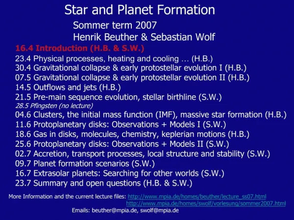
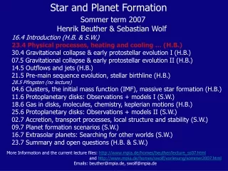
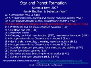
Star and Planet Formation Sommer term 2007 Henrik Beuther & Sebastian Wolf 16.4 Introduction (H.B. & S.W.) 23.4 Physical processes, heating and cooling, radiation transfer (H.B.) 30.4 Gravitational collapse & early protostellar evolution I (H.B.) 07.5 Gravitational collapse & early protostellar evolution II (H.B.) 14.5 Protostellar and pre-main sequence evolution (H.B.) 21.5 Outflows and jets (H.B.) 28.5 Pfingsten (no lecture) 04.6 Clusters, the initial mass function (IMF), massive star formation (H.B.) 11.6 Protoplanetary disks: Observations + models I (S.W.) 18.6 Gas in disks, molecules, chemistry, keplerian motions (H.B.) 25.6 Protoplanetary disks: Observations + models II (S.W.) 02.7 Accretion, transport processes, local structure and stability (S.W.) 09.7 Planet formation scenarios (S.W.) 16.7 Extrasolar planets: Searching for other worlds (S.W.) 23.7 Summary and open questions (H.B. & S.W.) More Information and the current lecture files: http://www.mpia.de/homes/beuther/lecture_ss07.html and http://www.mpia.de/homes/swolf/vorlesung/sommer2007.html Emails: beuther@mpia.de, swolf@mpia.de
Summary last week • Isothermal sphere, Lane-Emden equation, density profile of SIS r µ r-2 • Bonnor-Ebert mass = Jeans mass • MBE = MJ = m1at3/(r01/2G3/2) = 1.0Msun (T/(10K))3/2 (nH2/(104cm-3)-1/2 • Jeans length lJ = (pat2/Gr0)= 0.19pc (T/(10K))1/2 (nH2/(104cm-3)-1/2 - Virial theorem: 1/2 (d2I/dt2) = 2T + 2U + W + M If T, U and M very small, one can calculate free-fall time: tff = (3p/32Gr)1/2 • Thermal energy U to small to counteract gravity, but magnetic energy • M turns out to be important. • Many clouds in virial equlibrium 2T = -W • virial velocity: vvir = (Gm/r)1/2 • virial mass: mvir = v2r/G • Rotational energy not sufficient for cloud support • Rotation and magnetic field can increase critical masses for collapse and • fragmentation but magnetic field far more important. • --> if core mass below magnetically critical mass, core may be stable • against collapse even with increased outer pressure.
Virial Analysis • The generalized equation of hydrostatic equlibrium including magnetic • fields B acting on a current j and the full convective fluid velocity v is: • r Dv/Dt = -grad(P) - r grad(Fg) + 1/c j x B • Employing the Poisson equation and requiring mass conservation, one • gets after repeated integrations the VIRIAL THEOREM • 1/2 (d2I/dt2) = 2T + 2U + W + M • I: Moment of inertia, this decreases when a core is collapsing (m*r2) • T: Kinetic energy U: Thermal energy W: Gravitational energy M: Magnetic energy • All terms except W are positive. To keep the cloud stable, the other forces • have to match W. Dv/Dt=(∂v/∂t)x+(v grad)v 1/2(∂2I/∂t2) -2T 2U W M (Dv/Dt includes the rate of change at fixed spatial position x (∂v/∂t)x and the change induced by transporting elements to new location with differing velocity.)
Application of the Virial Theorem If all forces are too weak to match the gravitational energy, we get 1/2 (d2I/dt2) = W ~ -Gm2/r If the cloud complexes are in approximate force equilibrium, the moment of inertia actually does not change significantly and hence 1/2 (d2I/dt2)=0 2T + 2U + W + M = 0 This state is called VIRIAL EQUILIBRIUM.
z Ambipolar diffusion I In less dense GMCs, the ionization degree is relatively large and ions and neutrals are strongly collisionly coupled. Going to denser molecular cores, the ionization degree decreases, and neutrals and ions can easier decouple. Neutrals stream through the ions accelerated by gravity. There is a drag force between ions and neutrals from collisions. Furthermore, Lorentz force acts on ions. • The drift velocity between ions and neutrals is vdrift = vi - vn • And the drag force between ions and neutrals is: Fdrag = nn<sinvdrift>mnvdrift • (average number of collision per unit time nn<sinvdrift> times the transferred momentum mnvdrift) • The equation of motion with the Lorentz force is then: • niFdrag = j x B/c = 1/4π (rot B) x B • (with Ampere’s law: rot B = 4π/c * j) • vdrift = (rot B) x B / (4πninnmn <sinvdrift>) nn: neutral density ni: number of ions sin: ion-neutral cross section mn: mass of neutral
Ambipolar diffusion II • For a dense core with a size L, the time-scale for ambipolar diffusion is: • tad = L/|vdrift| = (4πninnmn <sinvdrift>)L / (|(rot B) x B|) Approximating |(rot B) x B| = B2/L we get tad = (4πninnmn <sinvdrift>)L2 / B2 Hence ambipolar diffusion time-scale is proportional to ionization degree, density and size of the cloud, and inversely proportional to magnetic field. • tad ≈ 3x10⁶yr (nH2/104cm-3)3/2 (B/30µG)-2 (L/0.1pc)2 It is still much under discussion whether this time-scale sets the rate where star formation takes place or whether it is too slow and other processes like turbulence are required.
z Ambipolar diffusion III Sequence of cloud equilibria can be described as continuous change of dM/dFB. The mass M enclosed by given flux FB (M(FB)) increases with time at fixed FB. For a centrally condensed core, the force balance can be approximated by 1/4π (rot B) x B = GMinnerr/w2 And one gets for the ambipolar diffusion time tad = w/|vdrift| = (4πninnmn <sinvdrift>)ww2/ (4πGMinnerr) = ni<sinvdrift>w3/(GMinner) In the central region for small ni w3 --> tad short, whereas further out with larger ni and larger radius w --> tad also increases
1.02x10⁷ yr 1.51x10⁷yr 1.60x10⁷yr 1.61x10⁷yr Ambipolar diffusion IV: Numerical modeling • Start with a uniform density cylinder and fixed boundary conditions. • Height of cylinder exceeds Jeans-length --> immediate collapse • After 6x10⁶yrs everything has settled in oblate configuration. • Then density increases due to ambipolar diffusion. • At 1.5x10⁷yrs, surface density that high that collapse accelerates. • --> Collapsing cloud core effectively separates from outer cloud. • B at the center increases.
Magnetic reconnection • Field lines of opposite direction are dragged together • --> antiparallel B field lines annihilate and magnetic energy is • dissipated as heat. • This process was first invoked to explain large luminosities observed • in solar flares.
Girart et al. 2006 Ambipolar diffusion caveat • Star Formation timescale: Observations indicate rapid star formation • on the order 1-2 million years. Ambipolar diffusion usually requires • longer cloud life-times. • Maybe gravo-turbulent fragmentation necessary
k=2 large-scale k=4 intermediate scale k=8 small scale MacLow 1999 Interstellar Turbulence • Supersonic --> creates network • of shocks • Shock interactions create density • fluctuations dr µ M2 which can • be relatively quiescent. • In these higher-density regions, • H and H2 may form rapidly • tform = 1.5x10⁹yr / (n/1cm-3) • (Hollenbach et al. 1971) • --> either molecular clouds form • slowly in low-density gas or • rapidly in ~105yr in n=104cm-3 • Decays on time-scales of order • the free-fall time-scale • --> needs to be replenished and • continuously driven • Candidates: Protostellar outflows, • radiation from massive stars, • Supernovae explosions
Gravo-turbulent fragmentation Klessen 2001 Freely decaying tubulence field Driven turbulence with wave- number k (perturbations l= L/k) 2 phases: -- Turbulent fragmentation -- Collapse of individual gravitational unstable cores Resulting clumb-mass spectra resembling the stellar initial mass function.
Simulation example SPH simulation with gravity and super- sonic turbulence. Initial conditions: Uniform density 1000Msun 1pc diameter Temperature 10K
Collapse of a core I Shu 1977 Ward-Thompson et al. 1999 µ r-2 Motte et al. 1998 Initial conditions: spherical self-gravitating isothermal sphere, simplified without magnetic field and rotation reaches rµ r-2
Collapse of a core II Log10(r) [g cm-3] Log10(|u|) [cm s-1] Log10(r) [cm] Log10(r) [cm] Important equations: Mass within radius r: Mr = ∫4πr2rdr --> ∂Mr/∂r = 4πr2r Continuity equation: ∂r/∂t = -1/r2 ∂(r2ru)/∂r u: velocity --> ∂Mr/∂t = -4πr2ru Hydrostatic momentum eq.: ∂u/∂t + u∂u/∂r = -1/r grad(P) - grad(F) With P = rat2for the ideal isothermal gas and grad(F) = -GMr/r2 ∂u/∂t + u∂u/∂r = -at2/r ∂r/∂r - GMr/r2 This set of equations can be solved numerically for given boundary conditions. • After forming a • central hydrostatic • core --> protostar, • the collapse starts • from the inside-out. • Density and velocity • profile in the inner • free-fall region • rµ r-3/2 & u µ r-1/2 • Density profile in the • outer envelope • rµ r-2 Singular isothermal sphere (Shu 1977)
Collapse of a core III . Mass accretion rate: M = ∂Mr/∂t = lim -4πr2ru = m0 at3/G r--> 0 For a typical sound speed of 0.2km/s at T=10K: M ~ 2 x 10⁻⁶ x(T/10K) Msun/yr --> Hence 1Msun star would form in 5 x 10⁵ yr. Using different initial conditions, e.g. Bonnor-Ebert spheres, one can get: . Myers 2005 For a singular isothermal sphere (SIS) one gets One finds an initial free-fall phase until the protostar has formed. Then the collapse continues in an inside-out mode but with varying accretion rate.
Collapse of a core IV The inner free-falling gas causes an inner pressure decrease, and a rarefaction wave moves outward. Within the rarefaction wave, the gas is free-falling because of missing pressure support.
The gravitational energy released per unit accreted mass can be approximated by the gravitational potential GM*/R* (with M* and R* the mass and radius of the central protostar) Hence the released accretion luminosity of the protostar can be approximated by this energy multiplied by the accretion rate: Lacc = GMM*/R* = 61Lsun (M/10-5Msun/yr) (M*/1Msun) (R*/5Rsun)-1 . . Accretion shock and Accretion luminosity
Rotational effects I Centrifugal force: Fcen= j2/w3 Gravitational force: Fgrav = Gm/w2 (w radius on cylindrical coordinates; j angular momentum j=mw2v) Since the initial ratio of rotational to gravitational energy is Trot/W ≈ 10-3 Rotation gets important after shrinkage of the core by a factor 1000. However, this is only valid in non-magnetic cloud. B-field anchored to rarified outer cloud. Spin-up twists the field, increases magn. tension and creates magn. torque counteracting spin-up. --> magnetic breaking: dense cores approximately corotate with cloud.
Rotational effects II • In dense core centers magnetic bracking fails because neutral matter • and magnetic field decouple with decreasing ionization fraction. • matter within central region can conserve angular momentum. Since grows faster than Fgrav each fluid element veers away from geometrical center. --> Formation of disk • The larger the initial angular momentum j of a fluid element, the further • away from the center it ends up --> centrifugal radius wcen • wcen = m03atW02t3/16 = 0.3AU (T/10K)1/2 (W0/10-14s-1)2 (t/105yr)3 wcen can be identified with disk radius. Increasing with time because in inside-out collapse rarefaction wave moves out --> increase of initial j.
Ovals are loci of constant line-of-sight for v(r) µ r-0.5 From Evans 1999 Infall signatures I Rising Tex along line of sight Velocity gradient Line optically thick An additional optically thin line peaks at center
Infall signatures II Models Spectra and fits (Myers et al. 1996) In a relatively simple model with two uniform regions along the line of sight with velocity dispersion s and peak optical depth t0, one can estimate the infall velocity vin: vin ≈ s2/(vred-vblue) * ln((1+eTBD/TD)/(1+eTRD/TD)) In low-mass regions vin is usually of the order 0.1 km/s.
Summary today • Ambipolar diffusion • Magnetic reconnection • Turbulence • Cloud collapse of singular isothermal sphere and Bonnor-Ebert sphere • Inside out collapse, rarefaction wave, density profiles, accretion rates • Accretion shock and accretion luminosity • Rotational effects, magnetic locking of “outer” dense core to cloud, • further inside it causes the formation of accretion disks • Observational infall signatures Important missing ingredients are molecular outflows and flattened Accretion disks --> subject of the next weeks.
Star and Planet Formation Sommer term 2007 Henrik Beuther & Sebastian Wolf 16.4 Introduction (H.B. & S.W.) 23.4 Physical processes, heating and cooling, radiation transfer (H.B.) 30.4 Gravitational collapse & early protostellar evolution I (H.B.) 07.5 Gravitational collapse & early protostellar evolution II (H.B.) 14.5 Protostellar and pre-main sequence evolution (H.B.) 21.5 Outflows and jets (H.B.) 28.5 Pfingsten (no lecture) 04.6 Clusters, the initial mass function (IMF), massive star formation (H.B.) 11.6 Protoplanetary disks: Observations + models I (S.W.) 18.6 Gas in disks, molecules, chemistry, keplerian motions (H.B.) 25.6 Protoplanetary disks: Observations + models II (S.W.) 02.7 Accretion, transport processes, local structure and stability (S.W.) 09.7 Planet formation scenarios (S.W.) 16.7 Extrasolar planets: Searching for other worlds (S.W.) 23.7 Summary and open questions (H.B. & S.W.) More Information and the current lecture files: http://www.mpia.de/homes/beuther/lecture_ss07.html and http://www.mpia.de/homes/swolf/vorlesung/sommer2007.html Emails: beuther@mpia.de, swolf@mpia.de