Download
1 / 18
320 likes | 610 Views
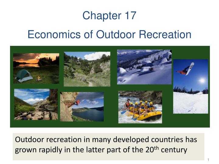
Chapter 17 Economics of Outdoor Recreation. Outdoor recreation in many developed countries has grown rapidly in the latter part of the 20 th century. snowmobiling. water skiing. cross-country skiing. horseback riding. Table 17-1, p.334.

E N D
Chapter 17 Economics of Outdoor Recreation Outdoor recreation in many developed countries has grown rapidly in the latter part of the 20th century
snowmobiling water skiing cross-country skiing horseback riding
Table 17-1, p.334 • Data for the U.S. on the number of people who participated in different types of outdoor recreation • Large percent increases in number of participants were in bird watching, hiking, backpacking, and sightseeing • Percent increases in number of participants in fishing and hunting were small • To some extent this may reflect the impacts of the environmental movement, which has tended to put greater emphasis on nonconsumptive uses of resources rather than the traditional consumptive uses • Traditionally, much of the supply of outdoor recreation resources has been a public function • In recent decades there has developed a privately provided market in outdoor recreation, from ski resorts to fishing and whale watching
1. The Demand for Outdoor Recreation Figure 17-1, p.335 • Demand curves for an imaginary public park: • Horizontal axis: visitor-days, defined as the total number of day-long visits (two half-day visits make one visitor-day); vertical axis: the entrance price to visit the park • There are a series of aggregate demand curves, each pertaining to a different time period (10 years ago, the current period, and 10 years in the future), arrived at by summing the individual demand curves of visitors to the park • q1, q2, and q3: numbers of visitor-days if entrance fees = 0 • Population growth, income growth, transportation improvements or drops in the price of gas, and taste and preference toward outdoor recreation shift D to the right
Efficient Visitation Rates Figure 17-2, p.337 • D is market demand curve for visits to a public park (MPB on slide 9 ) • D does not account for congestion externalities (MEB on slide 9)—when the rate of visitation increases, more visitors cause congestion that lowers the value of the visitation experience; if entrance fees are 0, there are open-access externalities—the users of the resource inflict on one another in the form of diminished resource value (q0: open-access level of visitation)
Efficient Visitation Rates (con’t) • Marginal costs of operating the park are constant at a level of MC (MSC on slide 9 ) • Curve A is MSB on slide 9 • MSB = MPB + MEB; MEB is negative though!!! • In order to lead to the socially efficient use rate q*, an extra fee = ‒MEB = congestion cost = C must be put into place • Total fee = MC + C
Modeling a Tax (on a negative consumption externality) $ tax = ‒MEB at QE MSC a Amount of tax b MPB MPBt MSB = MPB + MEB 0 QE QC Q ECO424-Ch7-slide 23
2. Rationing by Price • Rationing: the controlled distribution of scarce resources, goods, or services; rationing controls the size of the ration, one’s allotted portion of the resources being distributed on a particular day or at a particular time; in economics, rationing is an artificial restriction of demand • Rationing by price: charge an entrance fee sufficiently high that visitation is limited to q* • Nonprice rationing methods: limit entry to those people who meet some characteristics; first-come, first-served
P Percentage change in Qd Price elasticity of demand P1 = P2 Percentage change in P D Q Q1 Q2 15% = 1.5 10% 0 Pricing and Total Revenue Example: P rises by 10% Along a D curve, P and Q move in opposite directions, which would make price elasticity negative. We will drop the minus sign and report all price elasticities as positive numbers. Q falls by 15% Rule of thumb: The flatter the curve, the bigger the elasticity. The steeper the curve, the smaller the elasticity. Greg Mankiw’s Microeconomics-- CHAPTER 5 ELASTICITY AND ITS APPLICATION
% change in Q Price elasticity of demand = = % change in P P P1 P2 Q D Q1 Q2 0 “Inelastic demand” < 10% < 1 10% D curve: relatively steep P falls by 10% Consumers’ price sensitivity: relatively low Elasticity: < 1 Q rises less than 10% Greg Mankiw’s Microeconomics-- CHAPTER 5 ELASTICITY AND ITS APPLICATION
% change in Q Price elasticity of demand = = % change in P P P1 D P2 Q Q1 Q2 0 “Unit elastic demand” 10% = 1 10% D curve: intermediate slope Consumers’ price sensitivity: P falls by 10% intermediate Elasticity: 1 Q rises by 10% Greg Mankiw’s Microeconomics-- CHAPTER 5 ELASTICITY AND ITS APPLICATION
% change in Q Price elasticity of demand = = % change in P P P1 D P2 Q Q1 Q2 0 “Elastic demand” > 10% > 1 10% D curve: relatively flat Consumers’ price sensitivity: P falls by 10% relatively high Elasticity: > 1 Q rises more than 10% Greg Mankiw’s Microeconomics-- CHAPTER 5 ELASTICITY AND ITS APPLICATION
Percentage change in Q Price elasticity of demand = Percentage change in P 0 • If demand is elastic, then price elast. of demand > 1 % change in Q > % change in P • The fall in revenue from lower Q is greater than the increase in revenue from higher P, so revenue falls. Revenue = P x Q Greg Mankiw’s Microeconomics-- CHAPTER 5 ELASTICITY AND ITS APPLICATION
Percentage change in Q Price elasticity of demand = Percentage change in P 0 • If demand is inelastic, then price elast. of demand < 1 % change in Q < % change in P • The fall in revenue from lower Q is smaller than the increase in revenue from higher P, so revenue rises. Revenue = P x Q Greg Mankiw’s Microeconomics-- CHAPTER 5 ELASTICITY AND ITS APPLICATION
Differential Pricing Figure 17-6, p.345 • Many parks have capacity limits, either hard limits like a certain number of campsites or visitation levels where congestion externalities begin to take hold • Consider a park with a certain number of picnic sites q0; MC is constant; D1 is for weekday visitors and D2 is for weekend visitors • Two prices are required: during the week, set p1 = MC. But this price will not work for weekends, because quantity at this price will be q2 which exceeds the capacity q0; then set price = p2 during the weekends, thus total costs = c + d + e, total revenue = a + b + c + d + e, and profit = a + b, or, still charge p1 on the weekends, but with nonprice rationing
3. Ecotourism • A form of tourism involving visiting fragile, pristine, and relatively undisturbed natural areas, intended as a low-impact and often small scale alternative to standard commercial tourism • Its purpose may be to educate the traveler, to provide funds for ecological conservation, to benefit the economic development of local communities, or to foster respect for different cultures • Since the 1980s ecotourism has been considered a critical endeavor by environmentalists, so that future generations may experience destinations relatively untouched by human intervention