ESRI GIS Software
ESRI GIS Software. Data Types ESRI Data Model Shapefiles Raster Data Digital Orthophoto Quadrangle Digital Elevation Model Digital Raster Graphic ESRI GeoDatabase 2D Representations Registration Layering Accuracy Skewing & Size Registration Spatial Analysis United States

ESRI GIS Software
E N D
Presentation Transcript
Data Types ESRI Data Model Shapefiles Raster Data Digital Orthophoto Quadrangle Digital Elevation Model Digital Raster Graphic ESRI GeoDatabase 2D Representations Registration Layering Accuracy Skewing & Size Registration Spatial Analysis United States Inyo County City of Bishop 3D Representations Registration Overlaying Data Extraction Exporting to dbf Joins Attribute Joins Spatial Joins Join Types Examples 7.5-Minute Maps ESRI Limitations Contents
Shapefile Data • A shapefile stores nontopological geometry and attribute information for the spatial features in a data set. The geometry for a feature is stored as a shape comprising a set of vector coordinates. • Because shapefiles do not have the processing overhead of a topological data structure, they have advantages over other data sources such as faster drawing speed and edit ability. Shapefiles handle single features that overlap or that are noncontiguous. They also typically require less disk space and are easier to read and write. • Shapefiles can support point, line, and area features. Area features are represented as closed loop, double-digitized polygons. Attributes are held in a dBASE® format file. Each attribute record has a one-to-one relationship with the associated shape record.
Raster Data • Digital Orthophoto Quadrangle (DOQ) • A Digital Orthophoto Quadrangle (DOQ) is a digital, uniform-scale image created from aerial photos. It is a photographic map in which ground features are displayed in their true ground position because relief displacements caused by the camera and terrain of an aerial photograph have been removed. It combines the image characteristics of a photograph with the geometric qualities of a map; thus, it is possible to get direct measurements of distances, areas, angles, and positions from a DOQ.
Example (DOQ) • 7.5 Minute Quad-Triangle • Format MrSID • 1-Meter
Raster Data • Digital Elevation Model (DEM) • A Digital Elevation Model (DEM) is a digital cartographic/geographic dataset of elevations in xyz coordinates. The terrain elevations for ground positions are sampled at regularly spaced horizontal intervals. DEMs are derived from hypsographic data (contour lines) and/or photogrammetric methods using USGS 7.5-minute, 15-minute, 2-arc-second (30- by 60-minute), and 1-degree (1:250,000-scale) topographic quadrangle maps.
Example (DEM) • 7.5-Minute • Contour Lines • ESRI 3D Analyst
Raster Data • Digital Raster Graphic (DRG) • A Digital Raster Graphic (DRG) is a digital image (scanned version) of a USGS topographic map. DRGs are produced from USGS 1:24,000-, 1:24,000/1:25,000-, 1:63,360- (Alaska), 1:100,000-, and 1:250,000-scale topographic map series. The image inside the map neatline is georeferenced to the surface of the Earth and fit to the Universal Transverse Mercator (UTM) projection. The horizontal positional accuracy and datum of the DRG matches the accuracy and datum of the source map.
Example (DRG) • 7.5-Minute • Registration • Data Accuracy
ESRI GeoDatabase • Data Modification • Data Extraction • Tables • Relationships • Feature Classes
Quarter Quadrants NW NE SW SE
Rubberized Quadrants • Rubberizing Images • Image Registration • Image Locations (x,y) • Spatial Adjustment
Layering (Indian Reservations & Waters) Indian Reservation Lake
Layering (Roads) Indian Reservation Lake Roads
Data Accuracy • Images are available upto a accuracy of about 1-meter. • Common data characteristic are very important. • Time of capture data. • Data accuracy & size • Lens Skewing
DEM to TIN • Most DEM data contains the min and maximum elevation.
Adding Land & Waters Indian Reservation Lake
Complete All Layers Indian Reservation Roads Lake
Data Extraction • Shapefiles contain attributes for given data points, vectors, and polygons. • Data can be extracted directly into dbf format. • Spatial location is not directly exportable.
Joins • Like joining two tables by matching attribute values in a field, a spatial join appends the attributes of one layer to another. • You can then use the additional information to query your data in new ways. While you can also select features in one layer based on their location relative to another layer, a spatial join provides a more permanent association between the two layers because it creates a new layer containing both sets of attributes. • Several tables or layers can be joined to a single table or layer and relationship class joins can be mixed with attribute joins. • When a join table is removed, all data from tables that were joined after it are also removed, but data from previously joined tables remain. Symbology or labeling that is based on an appended column is returned to a default state when the join is removed. From: http://support.esri.com/articles
Spatial Joins • Join by location or spatial join uses spatial associations between the layers involved to append fields from one layer to another. Spatial joins are different from attribute and relationship class joins in that they are not dynamic and require the results to be saved to a new output layer. • Associations: One of three types of associations can be used to perform a spatial join. These associations are described as follows: • Match each feature to the closest feature or features - In this association, you can either append the attributes of the nearest feature or append an aggregate (i.e. min, max etc.) of the numeric attributes of the closest features. • Match each feature to the feature that it is part of - In this case, the attributes of the feature for which the current feature makes up a portion are appended. • Match each feature to the feature or features that it intersects - Like with the closest feature(s) association above, you can either append the attributes of a single intersecting feature or an aggregate of the numeric attributes of the intersecting features. From: http://support.esri.com/articles
Spatial Joins (Development & Programming) • Complex Queries: With VBA, however, it is possible to perform a join based on any association and with any combination of point, line or polygon feature layers. • Joins as well as other types of complex queries must be implemented using VBA or some other ESRI compliant language. • ESRI toolbox works primarily with Borland and Microsoft development products. Other languages can be used for development but are not well integrated due to the heavy usage of COM. From: http://support.esri.com/articles
Spatial Joins (Noted Points) • Noted Points: It is recommended that both layers have the same coordinate system. If the layers have different coordinate systems, the following rules apply: • The spatial join will be calculated in the target layer's (the select layer in the table of contents) coordinate system. • If the type of join performed involves adding a field to show the distance between joined features, the distance will be in a unit of measure associated with the target layer's coordinate system. • If one of the layers has an unknown coordinate system and the other a defined coordinate system, an error message will appear. If both layers have an unknown coordinate system, the join will proceed and the resulting layer will have an unknown coordinate system. • The coordinate system used to display data in ArcMap has no effect on how the data is joined. ArcMap allows data to be stored in one coordinate system and displayed in another. The analysis is always performed using the stored coordinate system. From: http://support.esri.com/articles
Spatial Join (Data Tables) Joined Data
Single & Multiple Spatial Joins The “Roads” layer is not spatially joined to “County”, and does not have a attribute which can relate location between them. The “Waters” layer does not contain a spatial relationship with the “Counties” layer, therefore any queries based on counties will not be applicable. • Multiple spatial joins are commonly needed to create relationships between many different layers.
Multiple Spatial Joins (Cont.) • By spatially joining the all the layers with the layer “Counties” we are able to create a spatial relationship between all the layers and the county they are located in.
Queries & Selections • Now that we have relations between the different layers, in order to take advantage of them, queries can be used to extract and filter data to find relevant spatial information.
Lakes Within One Mile of a Landmark (Visual Results) Landmarks that are within a mile from a body of water. • Layers which contain common relationship can be queried based upon these relationships as well as there own table attributes.
Lakes Within One Mile of a Landmark (Data Results) • Layers which contain common relationship can be queried based upon these relationships as well as there own table attributes.
Lakes Within One Mile of a Landmark • Layers which contain common relationship can be queried based upon these relationships as well as there own table attributes.
Lakes Within One Mile of the Road Roads that are within a mile from a body of water. • The returned table contains a filtered subset of the original roads, which are in Bishop and within one at most one mile from a body of water.
Lakes Within One Mile of the Road • The returned table contains a filtered subset of the original roads, which were in Bishop with roads which are now only within one mile of lakes.
Lakes Within One Mile of the Road • The returned table contains a filtered subset of the original roads, which were in Bishop with roads which are now only within one mile of lakes.