Testing Contingency Tables: Chi-Square Methods
Learn how to use Chi-square tests on contingency tables to assess relationships between variables, independence, and proportions in different populations. Practical examples and step-by-step guide included.

Testing Contingency Tables: Chi-Square Methods
E N D
Presentation Transcript
11.2 Tests Using Contingency Tables • When data can be tabulated in table form in terms of frequencies, several types of hypotheses can be tested by using the chi-square test. • The test of independence of variables is used to determine whether two variables are independent of or related to each other when a single sample is selected. • The test of homogeneity of proportions is used to determine whether the proportions for a variable are equal when several samples are selected from different populations. Bluman, Chapter 11
Test for Independence • The chi-square goodness-of-fit test can be used to test the independence of two variables. • The hypotheses are: • H0: There is no relationship between two variables. • H1: There is a relationship between two variables. • If the null hypothesis is rejected, there is some relationship between the variables. Bluman, Chapter 11
Test for Independence • In order to test the null hypothesis, one must compute the expected frequencies, assuming the null hypothesis is true. • When data are arranged in table form for the independence test, the table is called a contingency table. Bluman, Chapter 11
Contingency Tables • Cell • Row by column • The dimension of the contingency table is given: ROW by COLUMN Bluman, Chapter 11
Contingency Tables • The degrees of freedom for any contingency table are d.f. = (rows – 1) (columns – 1) = (R – 1)(C – 1). • The table above is 2 by 3. Only count the numerical cells. Bluman, Chapter 11
Test for Independence The formula for the test for independence: where d.f. = (R – 1)(C – 1) O = observed frequency E = expected frequency = Bluman, Chapter 11
Chapter 11Other Chi-Square Tests Section 11-2 Example 11-5 Page #606 Bluman, Chapter 11
Example (see page 618): College Education and Place of Residence A sociologist wishes to see whether the number of years of college a person has completed is related to her or his place of residence. A sample of 88 people is selected and classified as shown. At α= 0.05, can the sociologist conclude that a person’s location is dependent on the number of years of college? Bluman, Chapter 11
Example 11-5: College Education and Place of Residence Step 1: State the hypotheses and identify the claim. H0: A person’s place of residence is independent of the number of years of college completed. H1:A person’s place of residence is dependent on the number of years of college completed (claim). Step 2: Find the critical value. The critical value is 4.605, since the degrees of freedom are (2 – 1)(3 – 1) = 2. Bluman, Chapter 11
See next two slides for calculator use. Compute the expected values. (11.53) (13.92) (9.55) (10.55) (12.73) (8.73) (5.73) (6.92) (8.35) Bluman, Chapter 11
[A] Enter Observed values as Matrix 1: 2nd x-1 [B] Enter Expected values as Matrix Bluman, Chapter 11
Test statistics : c2=3.005 Bluman, Chapter 11
College Education and Place of Residence Step 3: Compute the test value. Bluman, Chapter 11
College Education and Place of Residence Step 4: Make the decision. • Do not reject the null hypothesis, since 3.01<9.488. Step 5: Summarize the results. • There is not enough evidence to support the claim that a person’s place of residence is dependent on the number of years of college completed. Bluman, Chapter 11
Chapter 11Other Chi-Square Tests Section 11-2 Example 11-6 Page #608 Bluman, Chapter 11
Example 11-6: Alcohol and Gender A researcher wishes to determine whether there is a relationship between the gender of an individual and the amount of alcohol consumed. A sample of 68 people is selected, and the following data are obtained. At α= 0.10, can the researcher conclude that alcohol consumption is related to gender? Bluman, Chapter 11
Example 11-6: Alcohol and Gender Step 1: State the hypotheses and identify the claim. H0: The amount of alcohol that a person consumes is independent of the individual’s gender. H1:The amount of alcohol that a person consumes is dependent on the individual’s gender (claim). Step 2: Find the critical value. The critical value is 9.488, since the degrees of freedom are (3 – 1 )(3 – 1) = (2)(2) = 4. Bluman, Chapter 11
Example 11-6: Alcohol and Gender Compute the expected values. (9.13) (9.93) (7.94) (13.87) (15.07) (12.06) Bluman, Chapter 11
Example 11-6: Alcohol and Gender Step 3: Compute the test value. Bluman, Chapter 11
Example 11-6: Alcohol and Gender Step 4: Make the decision. Do not reject the null hypothesis, since 0.283 < 4.605. . Step 5: Summarize the results. There is not enough evidence to support the claim that the amount of alcohol a person consumes is dependent on the individual’s gender. Bluman, Chapter 11
Test for Homogeneity of Proportions • Homogeneity of proportions test is used when samples are selected from several different populations and the researcher is interested in determining whether the proportions of elements that have a common characteristic are the same for each population. Bluman, Chapter 11
Test for Homogeneity of Proportions • The hypotheses are: • H0: p1 = p2 = p3 = … = pn • H1: At least one proportion is different from the others. • When the null hypothesis is rejected, it can be assumed that the proportions are not all equal. Bluman, Chapter 11
Assumptions for Homogeneity of Proportions • The data are obtained from a random sample. • The expected frequency for each category must be 5 or more. Bluman, Chapter 11
Chapter 11Other Chi-Square Tests Section 11-2 Example 11-7 Page #610 Bluman, Chapter 11
Example 11-7: Lost Luggage A researcher selected 100 passengers from each of 3 airlines and asked them if the airline had lost their luggage on their last flight. The data are shown in the table. At α= 0.05, test the claim that the proportion of passengers from each airline who lost luggage on the flight is the same for each airline. Bluman, Chapter 11
Example 11-7: Lost Luggage Step 1: State the hypotheses. H0: p1 = p2 = p3 = … = pn H1:At least one mean differs from the other. Step 2: Find the critical value. The critical value is 5.991, since the degrees of freedom are (2 – 1 )(3 – 1) = (1)(2) = 2. Bluman, Chapter 11
Example 11-7: Lost Luggage Compute the expected values. (7) (7) (7) (93) (93) (93) Bluman, Chapter 11
Example 11-7: Luggage Step 3: Compute the test value. Bluman, Chapter 11
Example 11-7: Lost Luggage Step 4: Make the decision. Do not reject the null hypothesis, since 2.765 < 5.991. . Step 5: Summarize the results. There is not enough evidence to reject the claim that the proportions are equal. Hence it seems that there is no difference in the proportions of the luggage lost by each airline. Bluman, Chapter 11
On your own • Read section 11.2 and all its examples. • Sec 11.2 page 614 • #1-7 all; • And #9, 17, 23, 27, 31 Bluman, Chapter 11