Download
1 / 20
200 likes | 355 Views
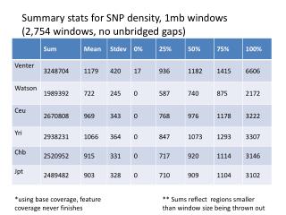
Summary stats for SNP density, 1mb windows (2,754 windows, no unbridged gaps). *using base coverage, feature coverage never finishes. ** Sums reflect regions smaller than window size being thrown out. SNP density 100kb windows (28,442). dbSNP 126 has 12million SNPs, including randoms , etc.

E N D
Summary stats for SNP density, 1mb windows (2,754 windows, no unbridged gaps) *using base coverage, feature coverage never finishes ** Sums reflect regions smaller than window size being thrown out
SNP density 100kb windows (28,442) dbSNP 126 has 12million SNPs, including randoms , etc. The region with the most SNPs is chr16 44943302-45043302
Regions with no SNPs (100kb) • Watson and Venter have 121 regions in common (292 & 162) • All HapMap has 444 in common (469-487) • They all have 111 in common • dbSNP has entries in these regions • Ensembl has a few Watson SNPs and many Venter SNPs (only 2 in chrY remained 0) here
Genome Graphs import uses a 10kb window for computing depth and coverage. For these graphs depth was chosen and connections were drawn between items up to 1mb away. Ceu was done with both 1mb connections and 10kb connections and there wasn’t a noticeable difference.
Allele comparisons Percent = (matches/total SNPs)*100 Total SNPs is Watson or Venter 1 or more includes the exact matches
Coding SNPs (RefSeq Genes) • Watson • 857 substitutions • 779 in dbSNP 128 • 706 heterozygous • Venter • 13 frameshifts • 1 in dbSNP 128 • 13 heterozygous • 1109 substitutions • 1003 in dbSNP 128 • 648 heterozygous
Comparing Venter’s deletion to alignments • 96,181 deletions • Extracted maf for +- 2bps of deletions • Found no deletions in other species at the same locations • Found from 0 to 27 species with alignments • Mean 2 per deletion, median 1, max 27 • chr9 36092117 36092118 A/-
Watson homozygous? SNPs • Only 1 allele found, not guaranteed homozygous • Found 382024 SNPs • matching species: min 0, max 27 (2 SNPs), ave 3, median 2 • 18,935 with 10 or more species • aligned but not matching: min 0, max 27 (2 SNPs), ave 3, median 2 • 25,663 with 10 or more species
Venter Homozygous? SNPs • Only 1 allele found, not guaranteed homozygous • 1,450,836 SNPs • matching species: min 0, max 27 ,ave 3, median 2 • aligned but not matching: min 0, max 27, ave 3, median 2