Trees
760 likes | 1.21k Views
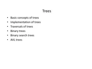
Trees. Basic concepts of trees Implementation of trees Traversals of trees Binary trees Binary search trees AVL trees. NOMOS Inc. R&D. Sales. Purchasing. Manufacturing. International. Domestic. Africa. Europe. Asia. Australia. Examples: Trees. A tree represents a hierarchy

Trees
E N D
Presentation Transcript
Trees • Basic concepts of trees • Implementation of trees • Traversals of trees • Binary trees • Binary search trees • AVL trees
NOMOS Inc. R&D Sales Purchasing Manufacturing International Domestic Africa Europe Asia Australia Examples: Trees • A tree represents a hierarchy • Organization structure of a corporation • A UNIX file system A B
What Is a Tree? • A tree is a collection of nodes. • The collection may be empty, i.e., without any node. • A non-empty tree has a node r, called the root, and zero or more nonempty (sub)trees T1, T2, …, Tk. The root of each subtree is connected by a directed edge from r.
Children and Parents • The root of each subtree is said to be a child of r • r is the parent of each subtree root. • From the recursive definition, we know that a tree is a collection of N nodes, one of which is the root, and N-1 edges. (Why N-1 edges?) Each edge connects some node to its parent, and every node except the root has one parent.
Leaves and Siblings • Each node may have an arbitrary number of children, possibly zero. • Nodes with no children are known as leaves. • Nodes with the same parent are siblings.
Paths • A path from node n1 to nk is defined as a sequence of nodes n1, n2, …, nk such that ni is the parent of ni+1 for 1 <= i < k. • The length of a path is the number of edges on the path. • There is a path of length zero from every node to itself. • How many paths are there from the root to each node in a tree?
Depth and Height • For any node ni, the depth of ni is the length of the unique path from the root to ni. • The depth of the root is 0. • The height of ni is the length of the longest path from ni to a leaf. • All leaves are at height 0. • The height of a tree is equal to the height of the root. • The depth of a tree is equal to the depth of the deepest leaf; this is always equal to the height of the tree.
Ancestors and Descendants • If there is a path from n1 to n2, then n1 is an ancestor of n2 and n2 is a descendant of n1. • If there is a path from n1 to n2 and n1 n2, then n1 is an proper ancestor of n2 and n2 is a proper descendant of n1.
Implementation of Trees • One way to implement a tree would be to have in each node, besides its data, a link to each child of the node. (Any problem?) • Wasted space: Since the number of children per node can vary so greatly and is not known in advance, it might be infeasible to make the children direct links in the data structure.
Node E has both a link to a sibling (F) and a link to a child (I) Implementation of Trees (cont.) • Another solution: Keep the children of each node in linked list of tree nodes. struct TreeNode { Object element; TreeNode *firstChild TreeNode *nextSibling; } nextSibling element firstChild Arrows that point downward are firstChild links. Arrows that go left to right are nextSibling links. Leaf nodes have neither siblings nor children.
N / / Implementation of Trees (cont.) · · A / B / C / D E F G / M / / H / / I / J / K / L / P / Q / /
Tree Traversals • Preorder traversal: In a preorder traversal, the work at a node is performed before (pre) its children are processed. • Postorder traversal: In a postorder traversal, the work at a node is performed after (post) its children are evaluated.
Preorder Traversal • In a preorder traversal, the work at a node is performed before (pre) its children are processed. PreOrder ( r ) { “visit” node r; //do what we need to do for each child w of rdo recursively perform PreOrder(w); } • Reading a document from beginning to end
Postorder Traversal • In a postorder traversal, the work at a node is performed after (post) its children are evaluated. PostOrder ( r ) { for each child w of rdo recursively perform PostOrder(w); “visit” node r; //do what we need to do } • du (disk usage) command in UNIX
root TL TR B C D E Binary Trees • A binary tree is a tree in which no nodes can have more than two children. • An important property of a binary tree is that the average depth of a binary tree is considerably smaller than N. • The average depth of a binary tree is O( ). • The average depth of a binary search tree is O(logN). • In the worst case, the depth can be as large as N-1. Both TL and TR could be possibly empty. A
left element right Implementation of Binary Trees • Since a binary tree has at most two children, we can keep direct links to them. struct BinaryNode { Object element; // The data in the node BinaryNode * left; // Left child BinaryNode * right; // Right child } • Applications: • Binary expression trees • Binary search trees How many NULL links are there in a binary tree with N nodes? 2N links; N-1 edges each corresponding one link N+1 NULL links
An Example: Expression Trees • An expression tree for (a+b*c)+((d*e+f)*g) • The leaves of an expression tree are operands (constants or variable names). • The internal nodes contain operators. • We can evaluate an expression tree, T, by applying the operator at the root to the values obtained by recursively evaluating the left and right subtrees. The left subtree evaluates to a+(b*c). The right subtree evaluates to ((d*e)+f)*g.
Inorder Traversal of Binary Trees • Inorder traversal of a binary tree InOrder ( r ) { recursively perform InOrder( left child of r ); “visit” node r; recursively perform InOrder( right child of r ); } • Producing an infix expression We can produce an (overly parenthesized) infix expression by recursively producing a parenthesized left expression, then printing out the operator at the root, and finally recursively producing a parenthesized right expression. ProduceInfixExp ( r ) { if r is a leaf then print (r->element); else print( ‘(‘ ); ProduceInfixExp( r->left); print( r->element ); ProduceInfixExp( r->right ); print( ‘)’ ); } ((a+(b*c))+(((d*e)+f)*g))
Traversals of Expression Trees • An inorder traversal of an expression tree produces its infix expression. • A postorder traversal of an expression tree produces its postfix expression. • A preorder traversal of an expression tree produces its prefix expression (the less useful). (a+b*c)+((d*e+f)*g) Postfix expression: abc*+de*f+g*+
Converting a Postfix Expression into an Expression Tree • The algorithm is similar to the postfix evaluation algorithm. • The algorithm • Read the postfix expression one symbol at a time. • If the symbol is an operand, create a one-node tree and push a pointer to it onto a stack. • If the symbol is an operator, pop (pointers) to two trees T1 and T2 (T2 is popped first) from the stack and form a new tree whose root is the operator and whose left and right children point to T1 and T2, respectively. A pointer to this new tree is then push onto the stack.
An Example: Constructing an Expression Tree • Input: ab+cde+** • The first two symbols are operands, so we create one-node trees and push pointers to them onto a stack. • Next, a + is read, so two pointers to trees are popped, a new tree is formed, and a pointer to it is pushed onto the stack.
An Example: Constructing an Expression Tree (cont.) • Input: ab+cde+** • Next, c, d, and e are read, and for each a one-node tree is created and a pointer to the corresponding tree is pushed onto the stack. • Now a + is read, so two trees are merged
An Example: Constructing an Expression Tree (cont.) • Input: ab+cde+** • Continuing, a * is read, so we pop two tree pointers and form a new tree with a * as root. • Finally, the last symbol is read, two trees are merged, and a pointer to the final tree is left on the stack.
Binary Search Trees • A Binary search tree is a binary tree such that any node has a key which is no less than the keys in its left subtree and no more than the keys in its right subtree. A binary search tree Not a binary search tree What is good about a binary search tree?
lt theElement rt The BinaryNode Class Constructor. Initializing the object as Grant the binary search tree class access to BinaryNode’s private data members.
BinarySearchTree class // ******************PUBLIC OPERATIONS********************* // void insert(Comparable x ) --> Insert x // void remove(Comparable x ) --> Remove x // Comparable find(Comparable x ) --> Return item that matches x // Comparable findMin( ) --> Return smallest item // Comparable findMax( ) --> Return largest item // boolean isEmpty( ) --> Return true if empty; else false // void makeEmpty( ) --> Remove all nodes in the tree // void printTree( ) --> Print tree in sorted order /** The tree root. */ private BinaryNode<Comparable> * root; const Comparable ITEM_NOT_FOUND; -> used if find operation fails // **PRIVATE OPERATIONS: Mostly Recursive********************* // Comparable elementAt( BinaryNode t) -> return the item (element) of node t // BinaryNode insert(Comparable x, BinaryNode t) -> insert x into the subtree whose root is t // BinaryNode remove(Comparable x, BinaryNode t) // BinaryNode find(Comparable x, BinaryNode t ) // BinaryNode findMin(BinaryNode t) // BinaryNode findMax(BinaryNode t) // void printTree(BinaryNode t ) A pointer to the root node; NULL for empty trees.
The Find Operation • The public member functions call private recursive functions to perform the operation. Call the internal find() to find the node containing x, return the item in that node by calling elementAt().
find()---Internal Member Function • This operation requires returning a pointer to the node in tree T that has item x, or NULL if there is no such node. Recursively find x in the left subtree. Recursively find x in the right subtree.
findMin() and findMax() • Return a pointer to the node containing the smallest and largest elements in the tree, respectively. • To perform a findMin, start at the root and go left as long as there is a left child. The stopping point is the smallest element. • To perform a findMax, start at the root and go right as long as there is a right child. The stopping point is the largest element.
findMin() and findMax() • Recursive implementation of findMin() • Non-recursive implementation of findMax() t is the left most node. Find the smallest item in the left subtree. Traverse down to the right most node.
insert() • Insert item x into the subtree whose root is t. Set the new root. Recursively insert into the left subtree. Recursively insert into the right subtree.
Issues about Insertion • Duplicates • Duplicates can be handled by keeping an extra field in the node record indicating the frequency of occurrence. • If the key is only part of a larger structure (data items may have the same key), we can keep all of the structures that have the same key in an auxiliary data structure, such as a list or another search tree.
remove() • If the node is a leaf, it can be deleted immediately. • If the node has one child, the node can be deleted after its parent adjusts a link to bypass the node.
remove() • If the node has two children, the general strategy is to replace the data of this node with the smallest data of the right subtree and recursively delete that node from the right subtree. • Lazy deletion: When an element is to be deleted, it is left in the tree and merely marked as being deleted. It is useful when the number of deletions is expected to be small. The node contains the smallest data of the right subtree. This node can be either a leaf node or a node with one child.
remove() Find the smallest item in the right subtree and replace the data item in node t with this item. t->element Deal with the cases when the item is in a leaf node or in a node with one child.
Destructor • We need to reclaim all memory occupied by the tree. Remove all nodes in the tree.
Copy Assignment Operator Reclaim all memory occupied by the tree Clone the tree of the right hand side of the assignment 1. Clone the left subtree. 2. Clone the right subtree. 3. Create a new node with left pointing to the left subtree and with right pointing to right subtree.
Average-Case Analysis for Binary Search Trees • Expect that all of the operations on binary search trees, except makeEmpty and operator=, should take O(lonN) time. • In constant time we descend a level in the tree • Operating on a tree is now roughly half as large • The running time of all operations (expect makeEmpty and operator=) is O(d), where d is the depth of the node containing the accessed item. • The average depth over all nodes in a tree is O(logN) on the assumption that all insertion sequences are equally likely. • The average running time of all operations (expect makeEmpty and operator=) is O(logN)
root TL TR Average Depth of Binary Search Trees • internal path length : The sum of the depths of all nodes in a tree. • Let D(N) be the internal path length for some tree T of N nodes. D(1) = 0. • An N-node tree consists of an i-node left subtree and (N-i-1)-node right subtree, plus a root at depth zero for 0 <= i < N. • D(i) is the internal path length of the left subtree w.r.t its root. In the main tree, all these nodes are one level deeper. • D(N-i-1) is the internal path length of the right subtree w.r.tits root. In the main tree, all these nodes are one level deeper. D(N) = D(i) + D(N-i-1) + N-1
root TL TR Average Depth of Binary Search Trees (cont.) • Let D(N) be the internal path length for some tree T of N nodes. D(1) = 0. D(N) = D(i) + D(N-i-1) + N-1 • The average value of both D(i) and D(N-i-1) is • Solving the above, we obtain D(N) = O(NlogN) • This implies that the expected depth is O(logN).
Solving D(N) Drop the insignificant –2 on the right, and divide the equation by N(N+1):
0 3 6 8 9 Solving D(N) (cont.) We obtain Then worst case:
7 1 2 7 3 4 1 4 2 5 5 3 9 8 8 8 2 1 AVL Trees • An AVL (Adelson-Velskii and Landis) tree is a binary search tree and for every node in the tree, the height of the left and right subtrees can differ by at most 1. Recall : The height of a tree is the length of the longest path from the root to a leaf. The height of an empty subtree is defined to be -1. 10
7 8 3 4 1 2 5 6 3 4 1 2 5 7 8 Inserting 6 Building AVL Trees • What is the problem? Inserting a node could violate the AVL tree property: for every node in the tree, the height of the left and right subtrees can differ by at most 1. • The property has to be restored before the insertion step is considered over. How? • Apply rotations to “balance” the tree
1 7 8 3 6 2 5 4 8 3 4 1 2 5 7 Inserting 6 Detect the Unbalanced Node • Nodes that are on the path from the insertion point to the root might have their balance altered. • Only those nodes have their subtrees altered. • Follow the path up to the root and update the balancing information, then we may find a node whose new balance violates the AVL condition. • Rebalance the tree at the first such node by rotations. 1 1 2 0 1 0
6 8 2 1 4 3 3 5 4 7 8 5 2 7 1 2 2 1 1 0 7.5 0 Inserting 6 Inserting 7.5 Four Violation Cases Denote by the node that must be rebalanced • An insertion into the left subtree of the left child of . • An insertion into the right subtree of the left child of . • An insertion into the left subtree of the right child of . • An insertion into the right subtree of the right child of .
k2 k1 k2 k1 k1 k2 Z Z Y Y X Y Z X X Single Rotation: fixes case 1) • Case 1): An insertion into the left subtree of the left child of . • Node k2 is the first node on the path up to the root that violates the AVL balance property. • Node k2 satisfies the AVL property before an insertion but violate it afterwards. • After insertion, subtree X has grown to an extra level, causing it to be exactly two levels deeper than Z. • Y cannot be at the same level as the new X because then k2 would have been out of balance before the insertion. • Y cannot be the same level as Z because then k1 would be the first node that violates the AVL balancing condition. after rotation before insertion after insertion The dashed lines mark the level
k2 k1 k2 k1 k1 k2 Z Z Y Y X Y Z X X Single Rotation: fixes case 1) (cont.) • Performing the single rotation: • k1 becomes the new root. • Since k2 >= k1, k2 becomes the right child of k1. • Z remains the right child of k2 • X remains the left child of k1 • Subtree Y is placed as k2’s left child after rotation before insertion after insertion The dashed lines mark the level
k2 k1 k1 k2 k1 k2 Z Y Y Z X X Single Rotation: fixes case 1) (cont.) • Essentially, X moves up one level, Y stays at the same level, and Z moves down one level. • k2 and k1 satisfy the AVL balance property, and have subtrees that are exactly the same height. • The new height of the entire subtrees is exactly the same as the height of the original subtree prior to the insertion that caused X to grow. • No further updating of heights on the path to the root is needed, and consequently no further rotations are needed. pivot Z Y X after rotation The dashed lines mark the level
7 2 1 4 3 8 7 5 5 5 1 4 3 8 2 6 8 6 7 3 4 1 2 k2 k1 k2 k1 1 1 Z Y Y Z 0 X X Examples: fixes case 1) after rotation 1 k2 2 k1 0 k2 k1 X 1 0 0 X 0 Inserting 6