Download
1 / 23
230 likes | 313 Views
Analyzing the decay of aftershock activities post Japanese and Sumatra earthquakes using the Generalized Omori's Law and Modified Bath's Law to establish parameter relationships and hypotheses. Applying AIC and maximum likelihood for hypothesis testing to determine the best fitting model. Results indicate Hypothesis II as the most suitable. The study covers 6 main shocks in Japan and Sumatra, utilizing earthquake catalogs and statistical methods to draw conclusions.

E N D
Aftershock Relaxation for Japanese and Sumatra Earthquakes Kazu Z. Nanjo1, B. Enescu2, R. Shcherbakov3, D.L. Turcotte3, T. Iwata1, & Y. Ogata1 1, ISM, Tokyo, Japan 2, Kyoto Univ., Kyoto, Japan 3, UC Davis, CA, USA
Objective: Analyze the decay of the aftershock activity for Japanese and Sumatra earthquakes, using catalogs maintained by Japan Meteorological Agency and Advanced National Seismic System. Approach: Generalized Omori’s law proposed by Shcherbakov et al. (2004, 2005).
The Gutenberg-Richter (GR) law (Gutenberg and Richter, 1954) • N: # of earthq. with mag. ≥ m • A and b: constants • The modified Bath’s law (Shcherbakov and Turcotte, 2004) Δm* = mms - m* m*: mag. of the inferred largest aftershock (m* = A/b) or mag. at the intercept between an extrapolation of the applicable GR law and N=1 mms: main shock mag.
The GR law can be rewritten for aftershocks as • The modified Omori’s law (Utsu, 1962) • dN/dt: rate of occurrence of aftershocks with mag. ≥m • t: time since the main shock • c and τ: characteristic times • p: exponent
Requirement among the parameters • Assume: • p is a constant independent of m and mms (Utsu, 1962) • b, mms, and Δm* are known parameters • Three possible hypotheses: • c is a constant c = c0 andτis dependent on m • τis a constant τ= τ0 and c is dependent on m • c and τ are dependent on m (Shcherbakov et al., 2004, 2005)
Hypoth. I, c = c0 • Hypoth. II, τ = τ0 • Hypoth. III, c and τ are dependent of m • c(m*): the characteristic time; β: a constant • Hypoth. III Hypoth. I if c(m*) = c0 and β = b • Hypoth. II if c(m*) = τ0(p-1) and β= bp
Spatial distribution and GR lawfor Kobe t (days) < 1000 A=4.85, b=0.78 m*=A/b=6.2 ( Mag. ≥ 2 t (days) < 1000 Δm*=1.1 mms=7.3 L (km) = 0.02 X 100.5m_ms [Kagan, 2002]
Aftershock relaxation for Kobe and small aftershocks in the early periods t (days) < 1000 0.01 ≤t < 0.1 0.1 ≤t < 1.0
How to find the best hypothesis • To find the optimal fitting of the prediction to the data for individual hypotheses • Point process modeling with max. likelihood (e.g., Ogata, 1983). • AIC (Akaike, 1974) to find the best hypothesis. AIC = -2(max. log-likelihood) + 2(# of parameters) • # of parameters • Hypoth. I: two (c0 and p) • Hypoth. II: two (τ0 and p) • Hypoth. III: three (c(m*), β, and p)
Test of the generalized Omori’s law for Kobe Hypoth. I, c = c0 Hypoth. II, τ=τ0 AIC=-3376.95 AIC=-3405.00 AIC=-3403.00 Hypoth. III, c and τare dependent on m
Aftershocks of Sumatra earthq. Mag. ≥ 4.5 t (days) < 251 t (days) < 251 A=8.88 b=1.20 m*=A/b=7.4 Δm*=1.6 ( mms=9.0
Test of the generalized Omori’s law for Sumatra Hypoth. I Hypoth. II AIC=-925.42 AIC=-936.76 Hypoth. III AIC=-934.76
Test of the generalized Omori’s law for Tottori Hypoth. I Hypoth. II AIC=-6630.54 AIC=-6654.70 Hypoth. III AIC=-6658.58
Establishment of the GR law (1) Kobe earthq. Hypoth. II c values for different m At time t = 0, dN/dt = 1/τ0 mms=7.3, b=0.78, Δm*=1.1 p=1.16, τ0=0.000508 (days)
Establishment of the GR law (2) Kobe t (days) < 1000, b=0.78 0.1 ≤t < 1.0, b=0.72 0.01 ≤t < 0.1, b=0.79
Establishment of the GR law (2) Kobe t (days) < 1000, b=0.78 0.1 ≤t < 1.0, b=0.72 0.01 ≤t < 0.1, b=0.79 Sumatra t (days) < 251, b=1.20 10 ≤t < 100, b=1.37 1.0 ≤t < 10, b=1.14 0.1 ≤t < 1.0, b=1.27 0.01 ≤t < 0.1, b=1.44
Conclusion • The generalized Omori’s law proposes: • Hypoth. I: τ scales with a lower cutoff mag. m and c is a constant. • Hypoth. II: c scales with m andτ is a constant. • Hypoth. III: Both c and τ scale with m. • 6 main shocks in Japan and Sumatra. • Earthq. catalogs of JMA and ANSS. • AIC and maximum likelihood to find the best hypoth. • The hypoth. II is best applicable to the entire sequence for different cutoff mag. from a state defined immediately after the main shock. • The c value is the characteristic time associated with the establishment of the GR law.
Test of the generalized Omori’s law for Niigata Hypoth. I Hypoth. II AIC=-7151.79 AIC=-7169.11 Hypoth. III AIC=-7167.16
Summary of parameter values m* = A/b Δm* = mms- masmax Δm* = mms- m*
Hypothesis I, c = c0 • Hypothesis II, τ = τ0 • Hypothesis III, c and τ are dependent of m (Shcherbakov et al., 2004, 2005) • c(m*): the characteristic time; β: a constant
Outline • Introduction of the generalized Omori’s law • 6 main shocks considered in this study • 5 Japanese earthquakes • 1 Sumatra earthquake • Application of the law to these earthquakes • Methods to find optimal fitting to the observed aftershock decay • Examples of the application • Summary of the application • Discussion • Conclusion