Geology 727
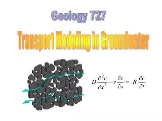
Geology 727. Transport Modeling in Groundwater. Subsurface Hydrology. Unsaturated Zone Hydrology. Groundwater Hydrology (Hydrogeology ). R = P - ET - RO. ET. ET. P. E. RO. R. waste. Water Table. Groundwater. v = q / = K I / . Processes we need to model

Geology 727
E N D
Presentation Transcript
Geology 727 Transport Modeling in Groundwater
Subsurface Hydrology Unsaturated Zone Hydrology Groundwater Hydrology (Hydrogeology)
R = P - ET - RO ET ET P E RO R waste Water Table Groundwater
v = q / = K I / • Processes we need to model • Groundwater flow • calculate both heads and flows (q) • Solute transport – requires information on flow (velocities) • calculate concentrations Darcy’s law
Types of Models • Physical (e.g., sand tank) • Analog (electric analog, Hele-Shaw) • Mathematical
Types of Solutions of Mathematical Models • Analytical Solutions: h= f(x,y,z,t) • (example: Theis eqn.) • Numerical Solutions • Finite difference methods • Finite element methods • Analytic Element Methods (AEM)
Finite difference models • may be solved using: • a computer programs (e.g., a FORTRAN program) • a spreadsheet (e.g., EXCEL)
Components of a Mathematical Model • Governing Equation • Boundary Conditions • Initial conditions (for transient problems) In full solute transport problems, we have two mathematical models: one for flow and one for transport. The governing equation for solute transport problems is the advection-dispersion equation.
Flow Code: MODFLOW • USGS code • finite difference code to solve the groundwater flow equation • MODFLOW 88 • MODFLOW 96 • MODFLOW 2000
Transport Code: MT3DMS • Univ. of Alabama • finite difference code to solve the advection-dispersion eqn. • Links to MODFLOW
The pre- and post-processor Groundwater Vistas links and runs MODFLOW and MT3DMS.
Introduction to solute transport modeling and Review of the governing equation for groundwater flow
Conceptual Model A descriptive representation of a groundwater system that incorporates an interpretation of the geological,hydrological, and geochemical conditions, including information about the boundaries of the problem domain.
Toth Problem Head specified along the water table Groundwater divide Groundwater divide Homogeneous, isotropic aquifer Impermeable Rock 2D, steady state
Toth Problem with contaminant source Contaminant source Homogeneous, isotropic aquifer Groundwater divide Groundwater divide Impermeable Rock 2D, steady state
Processes to model • Groundwater flow • Transport • Particle tracking: requires velocities and a particle tracking code. calculate path lines • (b)Full solutetransport: requires velocites and a solute transport model. calculate concentrations
Topo-Drive Finite element model of a version of the Toth Problem for regional flow in cross section. Includes a groundwater flow model with particle tracking.
Toth Problem with contaminant source Contaminant source Groundwater divide Groundwater divide advection-dispersion eqn Impermeable Rock 2D, steady state
v = q/n = K I / n • Processes we need to model • Groundwater flow • calculate both heads and flows (q) • Solute transport – requires information on flow (velocities) • calculate concentrations Requires a flow model and a solute transport model.
Groundwater flow is described by Darcy’s law. This type of flow is known as advection. Linear flow paths assumed in Darcy’s law True flow paths The deviation of flow paths from the linear Darcy paths is known as dispersion. Figures from Hornberger et al. (1998)
Advection-dispersion equation with chemical reaction terms. In addition to advection, we need to consider two other processes in transport problems. • Dispersion • Chemical reactions
Allows for multiple chemical species Dispersion Chemical Reactions Advection Source/sink term Change in concentration with time • is porosity; D is dispersion coefficient; v is velocity.
advection-dispersion equation groundwater flow equation
advection-dispersion equation groundwater flow equation
Flow Equation: 1D, transient flow; homogeneous, isotropic, confined aquifer; no sink/source term Transport Equation: Uniform 1D flow; longitudinal dispersion; No sink/source term; retardation
Flow Equation: 1D, transient flow; homogeneous, isotropic, confined aquifer; no sink/source term Transport Equation: Uniform 1D flow; longitudinal dispersion; No sink/source term; retardation
Assumption of the Equivalent Porous Medium (epm) REV Representative Elementary Volume
Dual Porosity Medium Figure from Freeze & Cherry (1979)
Review of the derivation of the governing equation for groundwater flow
General governing equation for groundwater flow Kx, Ky, Kz are components of the hydraulic conductivity tensor. Specific Storage Ss = V / (x y z h)
Law of Mass Balance + Darcy’s Law = Governing Equation for Groundwater Flow --------------------------------------------------------------- div q = - Ss (h t) +R* (Law of Mass Balance) q = - Kgrad h (Darcy’s Law) div (K grad h) = Ss (h t)–R*
Darcy column h/L = grad h Q is proportional to grad h q = Q/A Figure taken from Hornberger et al. (1998)
q = - Kgrad h K is a tensor with 9 components
Principal components of K Kxx Kxy Kxz KyxKyy Kyz Kzx KzyKzz K =
Darcy’s law q = - Kgrad h q equipotential line grad h q grad h Isotropic Kx = Ky = Kz = K Anisotropic Kx, Ky, Kz
global local z z’ x’ x Kxx Kxy Kxz Kyx Kyy Kyz Kzx Kzy Kzz K’x 0 0 0 K’y 0 0 0 K’z [K] = [R]-1 [K’] [R]
Law of Mass Balance + Darcy’s Law = Governing Equation for Groundwater Flow --------------------------------------------------------------- div q = - Ss (h t) +R* (Law of Mass Balance) q = - Kgrad h (Darcy’s Law) div (K grad h) = Ss (h t)–R*
V = Ssh (x y z) t t OUT – IN = x y z = change in storage = -V/ t Ss = V / (x y z h)
OUT – IN = = - V t
Law of Mass Balance + Darcy’s Law = Governing Equation for Groundwater Flow --------------------------------------------------------------- div q = - Ss (h t) +W* (Law of Mass Balance) q = - Kgrad h (Darcy’s Law) div (K grad h) = Ss (h t)–W*
2D confined: 2D unconfined: Storage coefficient (S) is either storativity or specific yield. S = Ss b & T = K b