Demand

1. Demand

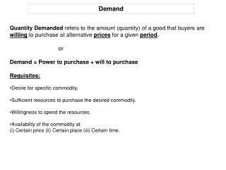
2. Deriving Demand Curves • An increase in the price of one good – holding tastes, income, and the price of other goods constant – causes a movement along the demand curve. • We use consumer theory to show how a consumer’s choice changes as the price changes, thereby tracing out the demand curve.

3. Deriving Demand Curves • In the previous chapter, we used calculus to maximize utility subject to a budget constraint. • We solved for the optimal quantities that a consumer chooses as a functions of prices and income. • We solved for the consumer’s system of demand functions for these goods.

4. Deriving Demand Curves • For example, Lisa chooses between pizzas, q1, and burgers, q2, so her demand functions are of the form • where p1is the price of pizza, and p2is the price of burger, and Y is her income.

5. Deriving Demand Curves • We showed that if a consumer has a Cobb-Douglas utility function • such demand functions are given by • Thus the Cobb-Douglas utility function has the unusual property that the demand function for each good depends only on its own price and not the price of the other good.

6. Deriving Demand Curves Illustration: Consider Michael, who consumes only beers, q1, and wines, q2. Let p1be the price of beers, p2be the price of wines, and Y is his income. We can derive his demand curve for beer by showing the quantities of beer he will purchase for some alternative prices of beer with price of wine and his income constant. Suppose that p2= 35 and Y = 420. Let us find q1for p1= 12, 6, and 4.

7. Deriving Demand Curves Wine (q2) 12.0 p2= 35 and Y= 420 Price-consumption curve e3 e2 5.5 I3 4.5 e1 I2 3.0 L3 (p1 =4) I1 L2 (p1 =6) L1 (p1 =12) 0 Beer (q1) 27 45 59 p1 E1 12 E2 6 E3 4 D1 0 Beer (q1) 27 45 59

8. Effects of an Increase in Income • An increase in an individual’s income, holding tastes and prices constant, causes a shift of the demand curve. • An increase in income causes a parallel shift of the budget constraint away from the origin, prompting a consumer to choose a new optimal bundle with more of some or all goods. • With price of beers fixed at p1= 12, and price of wines fixed at p2= 35, let us find q1for incomes, Y = 420, 630, and 840.

9. Wine (q2) p1= 12 and p2= 35 L3 (Y = 840) L2 (Y = 630) L1 (Y = 420) Income-consumption curve e3 7 e2 I3 5 e1 I2 3 I1 0 Beer (q1) 27 38 49 p1 E1 E2 E3 12 D3 D2 D1 0 Beer (q1) 27 38 49

10. Wine (q2) p1= 12 and p2= 35 L3 (Y = 840) L2 (Y = 630) L1 (Y = 420) Income-consumption curve e3 7 e2 I3 5 e1 I2 3 I1 0 Beer (q1) 27 38 49 Y Engel curve 840 E3 630 E2 420 E1 0 Beer (q1) 27 38 49

11. Wine (q2) Income-consumption curve e3 p1= 12 and p2= 35 20.5 L3 (Y = 840) I3 L2 (Y = 630) e2 11.5 if beer is an inferior good I2 L1 (Y = 420) e1 3.0 I1 0 Beer (q1) 10 19 27 Y E3 840 E2 630 420 E1 Engel curve 0 Beer (q1) 10 19 27

12. Effects of a Price Increase • Holding tastes, other prices, and income constant, an increase in a price of a good has two effects on an individual’s demand. • Substitution Effect • Income Effect

13. Substitution Effect • The change in the quantity of a good that a consumer demands when the good’s price rises, holding other prices and the consumer’s utility constant. • If utility is held constant as the price of the good increases, consumers substitute other, now relatively cheaper goods for that one.

14. Income Effect • The change in the quantity of a good a consumer demands because of a change in income, holding prices constant. • An increase in price reduces a consumer’s buying power, effectively reducing the consumer’s income or opportunity set and causing the consumer to buy less of at least some goods.

15. Income and Substitution Effects with a Normal Good q2 e* e2 e1 I1 I2 L2 L* L1 q1 0 6 10 16 Income effect Substitution effect Total effect

16. Income and Substitution Effects with a Normal Good • The total effect from the price change is the sum of the substitution and income effects. • Because indifference curves are convex to the origin, the substitution effect is unambiguous. • Less of a good is consumed when its price rises. • A consumer always substitutes a less expensive good for a more expensive one, holding utility constant.

17. Income and Substitution Effects with a Normal Good • The substitution effect causes a movement along an indifference curve. • The income effect causes a shift to another indifference curve due to a change in the consumer’s opportunity set. • The direction of the income effect depends upon the type of good. • Since the good is normal, the income effect is negative with respect to price increase. • Thus, both the substitution and income effect go in the same direction, so the total effect of the price increase must be negative.

18. Income and Substitution Effects with an Inferior Good q2 Assume q1 is an inferior good e* e1 e2 I1 I2 L2 L* L1 q1 0 10 12 16 Income effect Total effect Substitution effect

19. Income and Substitution Effects with an Inferior Good • If a good is inferior, the income effect goes in the opposite direction from the substitution effect. • For most inferior goods, the income effect is smaller than the substitution effect. • The total effect moves in the same direction as the substitution effect, but the total effect is smaller. • However, the income effect can more than offset the substitution effect in extreme cases.

20. Income and Substitution Effects with a Giffen Good • A good is called a Giffen good if an increase in its price causes the quantity demanded to rise. • Thus, the demand curve for a Giffen good slopes upward. • It was named after Robert Giffen, a 19th century British economist who argued that poor people in Ireland increased their consumption of potatoes when the price rose because of a potato blight.

21. Income and Substitution Effects with a Giffen Good q2 L* Assume q1 is a Giffen good L1 e* L2 e1 I1 e2 I2 q1 0 8 14 16 Substitution effect Total effect Income effect

22. Compensated Demand Curve • We could derive a compensated demand curve, where we determine how the quantity demanded changes as the price rises, holding utility constant. • The change in the quantity demanded reflects only pure substitution effects when the price changes. • It is called the compensated demand curve because we would have to compensate an individual – give the individual extra income – as the price rises so as to hold the individual’s utility constant.

23. Compensated Demand Curve • It is also called the Hicksian demand curve, after John Hicks, who introduced the idea. • The compensated demand function for q1 is • where we hold utility constant at • We cannot observe the compensated demand curve directly because we do not observe utility levels. • Because the compensated demand curve reflects only substitution effects, the Law of Demand must hold: A price increase causes the compensated demand for a good to fall.

24. Deriving Compensated Demand Curve q2 p2= 35 and Y= 420 12.0 e3 e1 e2 I1 I2 L1 (p1 =6) L2 (p1 =12) L* q1 0 27 41 45 p1 E3 E2 12 E1 6 Uncompensated Demand Curve (D) Compensated Demand Curve (H) q1 0 27 41 45

25. Deriving Compensated Demand Curve • We can also derive the compensated demand curve by using the expenditure function. • Differentiating the expenditure function with respect to p1, we obtain the compensated demand function for q1.

26. Deriving Compensated Demand Curve Illustration: Find the compensated demand function for q1 given a Cobb-Douglas utility function below with a = 0.6. The expenditure function for this Cobb-Douglas utility function is

27. Deriving Compensated Demand Curve Differentiating the expenditure function with respect to p1 we have the compensated demand function given as Given that a = 0.6, then the expenditure function becomes

28. Deriving Compensated Demand Curve The compensated demand function for q1 is