Selinger Optimizer
In this lecture, Sam Madden discusses the challenge of efficiently ordering a series of joins in database queries. The naive method of ordering joins leads to exponential complexity, making it impractical for large datasets. He presents an optimized approach using dynamic programming, where the minimum cost join orders are calculated based on previously computed access methods for each relation. The technique includes cache utilization and considerations for interesting orders that may enhance the final output, displaying a significant reduction in computational cost for complex joins.

Selinger Optimizer
E N D
Presentation Transcript
Selinger Optimizer 6.830 Lecture 10 October 15, 2009 Sam Madden
The Problem • How to order a series of N joins, e.g., A.a = B.b AND A.c = D.d AND B.e = C.f N! ways to order joins (e.g., ABCD, ACBD, ….) (N-1)! plans per ordering (e.g., (((AB)C)D), ((AB)(CD), …) Multiple implementations (e.g., hash, nested loops, etc) • Naïve approach doesn’t scale, e.g., for 20-way join • 10! x 9! = 1.3 x 10 ^ 12 • 20! x 19! = 2.9 x 10 ^ 35
Selinger Optimizations • Left-deep only (((AB)C)D) (eliminate (N-1)!) • Push-down selections • Don’t consider cross products • Dynamic programming algorithm
Dynamic Programming R set of relations to join (e.g., ABCD) For ∂ in {1...|R|}: for S in {all length ∂ subsets of R}: optjoin(S) = a join (S-a), where a is the single relation that minimizes: cost(optjoin(S-a)) + min. cost to join (S-a) to a + min. access cost for a optjoin(S-a) is cached from previous iteration
Cache Example optjoin(ABCD) – assume all joins are NL ∂=1 A = best way to access A (e.g., sequential scan, or predicate pushdown into index...) B = best way to access B C = best way to access C D = best way to access D Total cost computations: choose(N,1), where N is number of relations
Cache Example optjoin(ABCD) ∂=2 {A,B} = AB or BA (using previously computed best way to access A and B) {B,C} = BC or CB {C,D} = CD or DC {A,C} = AC or CA {A,D} = AD or DA {B,D} = BD or DB Total cost computations: choose(N,2) x 2
Cache Example optjoin(ABCD) ∂=3 {A,B,C} = remove A, compare A({B,C}) to ({B,C})A remove B, compare B({A,C}) to ({A,C})B remove C, compare C({A,B}) to ({A,B})C {A,B,D} = remove A, compare A({B,D}) to ({B,D})A …. {A,C,D} = … {B,C,D} = … Already computed – lookup in cache Total cost computations: choose(N,3) x 3 x 2
Cache Example optjoin(ABCD) ∂=4 {A,B,C,D} = remove A, compare A({B,C,D}) to ({B,C,D})A remove B, compare B({A,C,D}) to ({A,C,D})B remove C, compare C({A,B,D}) to ({A,B,D})C remove D, compare D({A,B,C}) to ({A,B,C})D Already computed – lookup in cache Final answer is plan with minimum cost of these four Total cost computations: choose(N,4) x 4 x 2
Complexity choose(n,1) + choose(n,2) + … + choose(n,n) total subsets considered All subsets of a size n set = power set of n = 2^n Equiv. to computing all binary strings of size n 000,001,010,100,011,101,110,111 Each bit represents whether an item is in or out of set
Complexity (continued) For each subset, k ways to remove 1 join k < n m ways to join 1 relation with remainder Total cost: O(nm2^n) plan evaluations n = 20, m = 2 4.1 x 10^7
Interesting Orders • Some queries need data in sorted order • Some plans produce sorted data (e.g., using an index scan or merge join • May be non-optimal way to join data, but overall optimal plan • Avoids final sort • In cache, maintain best overall plan, plus best plan for each interesting order • At end, compare cost of best plan + sort into order to best in order plan • Increases complexity by factor of k+1, where k is number of interesting orders
Example SELECT A.f3, B.f2 FROM A,B where A.f3 = B.f4 ORDER BY A.f3 compare: cost(sort(output)) + 156 to 180