Download
1 / 26
260 likes | 278 Views
Learn how to read and write data from different file types, including text files, images, and Excel files. Understand the basics of file input and output and how to structure code using pipelines for efficient data processing.

E N D
File Input and Output July 2nd, 2015
Inputs and Outputs • Inputs • Keyboard • Mouse • storage(hard drive) • Networks • Outputs • Graphs • Images • Videos(image stacks) • Text files • Statistical results
Keyboard Input • The simplest input is reading in lines from the user • print (“Please enter a number: “) x = scan() • Print (“Your number is “ + x)
Inputs and Outputs • Entering data on your own is time consuming • Large amounts of Data already exist in files • MATLAB, R, and Python all provide the ability to read data from files (as well as write data to files)
The basics of File Input and Output File Input and Output are the bread and butter of data manipulation and generation File Code New File
Part 1: File Types • Text Files • Images • Excel Files • FASTA files • Other
Text Files • A lot of data comes in the form of of spreadsheets in text files (.txt or .csv extension) • Generally the easiest to manipulate
Image files • Images are stored as spreadsheets, where each pixel is represented by an X and Y co-ordinate and a range of values for the intensity of the pixel • These values depend on what type of file the image is
Binary and Grayscale • Binary Image • Represented as either Boolean (TRUE, FALSE) or numerical (0,1) • Grayscale Image • Represented with a range of numerical values (usually between 0 and 255)
Binary and Grayscale Grayscale Binary
Color images • Color images can be thought of as a stack of 3 images (red, blue, green) • The intensity of each color is represented as a number between 0-255
Common I/O themes • File type – The type of file the data will be saved as. • Data type – The type (or mode) of the data (integers, strings, characters) • Separator: What separates the data from each other; in text files, this is often a ,
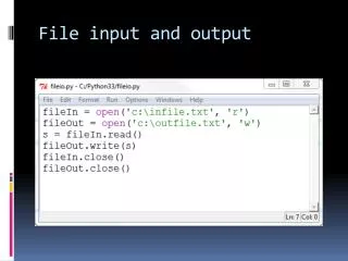
Reading a file • Most programming languages have functions that “read” files. • You generally have to specify the type of file being read, or the computer will not know how to interpret what it's looking at
Reading a File • Reading data into a program can often times be difficult and frustrating • Can sometimes take more time than the rest of the coding! • It's important to understand the subtleties and nuances that is specific to each language
“Data Preparation” • When working with any type of spread-sheet like files (e.g., excel): easier to export the data as a text file • Image files can be converted from one type to another with relative ease. How you want to manipulate an image will determine in what format you want to save the image as.
Character Encoding • Used to represent all of the characters in a form computers can understand it • There are different types of character coding, the most common being Unicode • Modern operating systems are likely to use UTF-8 or Unicode files
Character Encoding • If character encoding differs between your data and what a computer uses to view the data, your text files can look like gibberish. • Character Encoding can be changed using programming language specific functions
Reading a File • R • read.table() • read.csv • scan() • Python • .read() • open() • readline() • Matlab • importdata() • fscanf() • fopen()
File Output • Generating a file is an easier process than reading in a file • Stored data can be written to a file of your choosing, whether it's an image, text file, etc. • write(x, file = “C:\Program Files\R\data.txt”) • write(x, file = “data.txt”, sep = “,”)
The Working Directory • The working directory can be thought of as the area that the programming language currently points to • When reading or writing files, if a full path name is not given, the program will automatically look in the working directory to read or write a file
Part 2: Pipelines • A way of structuring code that makes it simple to work with • Simply, a pipeline is a chain of processes (such as functions) arranged so that the output of one process is the input to the next process
Part 2: Pipelines Sequence Data Find Start Codon Convert to Amino Acids Save Amino Acid File
Functions • findstart <- function(fullseq, codons = c("atg", "taa", "tag", "tga")){ startposition <- sapply(codons, function(x){start(matchPattern(x, fullseq))}) return(substr(sequence, startposition, length(fullseq)) } • AminoSequence ← function(sequence){ amino ← *lots of code and a library of amino acid sequences* return(amino) }
Functions • simplesequence ← scan(“simplesequence.txt”) • sequenceTwo ← findstart(Thesequence) • AminoSeq ←AminoSequence(sequenceTwo) • write.file(AminoSeq, file = “Amino.txt”)
Pipelines • Structuring your code into functions can help ease the readability of your code and allow you to reuse functions for similar processes • Pipelines are excellent for automatic processing of a large amount of data sets