Download
1 / 62
620 likes | 652 Views
Explore complex random effect models in epidemiology and ecology, including multivariate models and MCMC estimation. Discover applications in artificial insemination, Danish chicken examples, and great tit nesting behavior. Learn about efficient MCMC algorithms and future research directions.

E N D
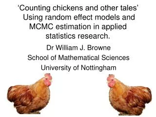
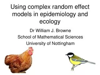
Using complex random effect models in epidemiology and ecology Dr William J. Browne School of Mathematical Sciences University of Nottingham
Outline • Background to my research, random effect and multilevel models and MCMC estimation. • Random effect models for complex data structures including artificial insemination and Danish chicken examples. • Multivariate random effect models and great tit nesting behaviour. • Efficient MCMC algorithms. • Conclusions and future work.
Background • 1995-1998 – PhD in Statistics, University of Bath. “Applying MCMC methods to multilevel models.” • 1998-2003 – Postdoctoral research positions at the Centre for Multilevel Modelling at the Institute of Education, London. • 2003-2006 – Lecturer in Statistics at University of Nottingham. • 2006-2007 Associate professor of Statistics at University of Nottingham. • 2007- Professor in Biostatistics, University of Bristol. Research interests: Multilevel modelling, complex random effect modelling, applied statistics, Bayesian statistics and MCMC estimation.
Random effect models • Models that account for the underlying structure in the dataset. • Originally developed for nested structures (multilevel models), for example in education, pupils nested within schools. • An extension of linear modelling with the inclusion of random effects. A typical 2-level model is Here i might index pupils and j index schools. Alternatively in another example i might index cows and j index herds. The important thing is that the model and statistical methods used are the same!
Estimation Methods for Multilevel Models Due to additional random effects no simple matrix formulae exist for finding estimates in multilevel models. Two alternative approaches exist: • Iterative algorithms e.g. IGLS, RIGLS, that alternate between estimating fixed and random effects until convergence. Can produce ML and REML estimates. • Simulation-based Bayesian methods e.g. MCMC that attempt to draw samples from the posterior distribution of the model. One possible computer program to use for multilevel models which incorporates both approaches is MLwiN.
MLwiN • Software package designed specifically for fitting multilevel models. • Developed by a team led by Harvey Goldstein and Jon Rasbash at the Institute of Education in London over past 15 years or so. Earlier incarnations ML2, ML3, MLN. • Originally contained ‘classical’ estimation methods (IGLS) for fitting models. • MLwiN launched in 1998 also included MCMC estimation. • My role in the team was as developer of the MCMC functionality in MLwiN in my time at Bath and during 4.5 years at the IOE. Note: MLwiN core team relocated to Bristol in 2005.
MCMC Algorithm • Consider the 2-level normal response model • MCMC algorithms usually work in a Bayesian framework and so we need to add prior distributions for the unknown parameters. • Here there are 4 sets of unknown parameters: • We will add prior distributions
MCMC Algorithm (2) One possible MCMC algorithm for this model then involves simulating in turn from the 4 sets of conditional distributions. Such an algorithm is known as Gibbs Sampling. MLwiN uses Gibbs sampling for all normal response models. Firstly we set starting values for each group of unknown parameters, Then sample from the following conditional distributions, firstly To get .
MCMC Algorithm (3) We next sample from to get , then to get , then finally To get . We have then updated all of the unknowns in the model. The process is then simply repeated many times, each time using the previously generated parameter values to generate the next set
Burn-in and estimates Burn-in: It is general practice to throw away the first n values to allow the Markov chain to approach its equilibrium distribution namely the joint posterior distribution of interest. These iterations are known as the burn-in. Finding Estimates: We continue generating values at the end of the burn-in for another m iterations. These m values are then averaged to give point estimates of the parameter of interest. Posterior standard deviations and other summary measures can also be obtained from the chains.
So why use MCMC? • Often gives better (in terms of bias) estimates for non-normal responses (see Browne and Draper, 2006). • Gives full posterior distribution so interval estimates for derived quantities are easy to produce. • Can easily be extended to more complex problems as we will see next. • Potential downside 1: Prior distributions required for all unknown parameters. • Potential downside 2: MCMC estimation is much slower than the IGLS algorithm. • For more information see my book: MCMC Estimation in MLwiN – Browne (2003).
School S1 S2 S3 S4 Pupil P1 P2 P3 P4 P5 P6 P7 P8 P9 P10 P11 P12 Nbhd N1 N2 N3 Extension 1: Cross-classified models For example, schools by neighbourhoods. Schools will draw pupils from many different neighbourhoods and the pupils of a neighbourhood will go to several schools. No pure hierarchy can be found and pupils are said to be contained within a cross-classification of schools by neighbourhoods:
Notation With hierarchical models we use a subscript notation that has one subscript per level and nesting is implied reading from the left. For example, subscript pattern ijk denotes the i’th level 1 unit within the j’th level 2 unit within the k’th level 3 unit. If models become cross-classified we use the term classification instead of level. With notation that has one subscript per classification, that also captures the relationship between classifications, notation can become very cumbersome. We propose an alternative notation introduced in Browne et al. (2001) that only has a single subscript no matter how many classifications are in the model.
i nbhd(i) sch(i) 1 1 1 2 2 1 3 1 1 4 2 2 5 1 2 6 2 2 School S1 S2 S3 S4 7 2 3 Pupil P1 P2 P3 P4 P5 P6 P7 P8 P9 P10 P11 P12 8 3 3 Nbhd N1 N2 N3 9 3 4 10 2 4 11 3 4 12 3 4 Single subscript notation We write the model as where classification 2 is neighbourhood and classification 3 is school. Classification 1 always corresponds to the classification at which the response measurements are made, in this case pupils. For pupils 1 and 11 equation (1) becomes:
Neighbourhood School Pupil Classification diagrams In the single subscript notation we lose information about the relationship (crossed or nested) between classifications. A useful way of conveying this information is with the classification diagram. Which has one node per classification and nodes linked by arrows have a nested relationship and unlinked nodes have a crossed relationship. School Neighbourhood Pupil Cross-classified structure where pupils from a school come from many neighbourhoods and pupils from a neighbourhood attend several schools. Nested structure where schools are contained within neighbourhoods
Donor Donation Woman Cycle Example : Artificial insemination by donor 1901 women 279 donors 1328 donations 12100 ovulatory cycles response is whether conception occurs in a given cycle In terms of a unit diagram: Or a classification diagram:
Parameter Description Estimate(se) intercept -4.04(2.30) azoospermia 0.22(0.11) semen quality 0.19(0.03) womens age>35 -0.30(0.14) sperm count 0.20(0.07) sperm motility 0.02(0.06) insemination to early -0.72(0.19) insemination to late -0.27(0.10) women variance 1.02(0.21) donation variance 0.644(0.21) donor variance 0.338(0.07) Model for artificial insemination data We can write the model as Results: Note cross-classified models can be fitted in IGLS but are far easier to fit using MCMC estimation.
Extension 2: Multiple membership models • When level 1 units are members of more than one higher level unit we describe a model for such data as a multiple membership model. • For example, • Pupils change schools/classes and each school/class has an effect on pupil outcomes. • Patients are seen by more than one nurse during the course of their treatment.
n1(j=1) n2(j=2) n3(j=3) p1(i=1) 0.5 0 0.5 p2(i=2) 1 0 0 p3(i=3) 0 0.5 0.5 p4(i=4) 0.5 0.5 0 Here patient 1 was seen by nurse 1 and 3 but not nurse 2 and so on. If we substitute the values of w(2)i,j, i and j. from the table into (2) we get the series of equations : Notation Note that nurse(i) now indexes the set of nurses that treat patient i and w(2)i,jis a weighting factor relating patient i to nurse j. For example, with four patients and three nurses, we may have the following weights:
nurse Here patients are multiple members of nurses, nurses are nested within hospitals and GP practice is crossed with both nurse and hospital. patient hospital nurse GP practice patient Classification diagrams for multiple membership relationships Double arrows indicate a multiple membership relationship between classifications. We can mix multiple membership, crossed and hierarchical structures in a single model.
Farm House Parent flock Child flock Example involving nesting, crossing and multiple membership – Danish chickens Production hierarchy 10,127 child flocks 725 houses 304 farms Breeding hierarchy 10,127 child flocks 200 parent flocks As a unit diagram: As a classification diagram:
Parameter Description Estimate(se) intercept -2.322(0.213) 1996 -1.239(0.162) 1997 -1.165(0.187) Results: hatchery 2 -1.733(0.255) hatchery 3 -0.211(0.252) hatchery 4 -1.062(0.388) parent flock variance 0.895(0.179) house variance 0.208(0.108) farm variance 0.927(0.197) Model and results Response is cases of salmonella Note multiple membership models can be fitted in IGLS and this model/dataset represents roughly the most complex model that the method can handle. Such models are far easier to fit using MCMC estimation.
Random effect modelling of great tit nesting behaviour • An extension of cross-classified models to multivariate responses. • Collaborative research with Richard Pettifor (Institute of Zoology, London), and Robin McCleery and Ben Sheldon (University of Oxford).
Wytham woods great tit dataset • A longitudinal study of great tits nesting in Wytham Woods, Oxfordshire. • 6 responses : 3 continuous & 3 binary. • Clutch size, lay date and mean nestling mass. • Nest success, male and female survival. • Data: 4165 nesting attempts over a period of 34 years. • There are 4 higher-level classifications of the data: female parent, male parent, nestbox and year.
Source Number of IDs Median #obs Mean #obs Year 34 104 122.5 Nestbox 968 4 4.30 Male parent 2986 1 1.39 Female parent 2944 1 1.41 Data background The data structure can be summarised as follows: Note there is very little information on each individual male and female bird but we can get some estimates of variability via a random effects model.
Univariate cross-classified random effect modelling • For each of the 6 responses we will firstly fit a univariate model, normal responses for the continuous variables and probit regression for the binary variables. For example using notation of Browne et al. (2001) and letting response yibe clutch size:
Estimation • We use MCMC estimation in MLwiN and choose ‘diffuse’ priors for all parameters. • We run 3 MCMC chains from different starting points for 250k iterations each (500k for binary responses) and use the Gelman-Rubin diagnostic to decide burn-in length. • We compared results with the equivalent classical model using the Genstat software package and got broadly similar results. • We fit all four higher classifications and do not consider model comparison.
Clutch Size Here we see that the average clutch size is just below 9 eggs with large variability between female birds and some variability between years. Male birds and nest boxes have less impact.
Lay Date (days after April 1st) Here we see that the mean lay date is around the end of April/beginning of May. The biggest driver of lay date is the year which is probably indicating weather differences. There is some variability due to female birds but little impact of nest box and male bird.
Nestling Mass Here the response is the average mass of the chicks in a brood at 10 days old. Note here lots of the variability is unexplained and both parents are equally important.
Human example Helena Jayne Browne Born 22nd May 2006 Birth Weight 8lb 0oz Sarah Victoria Browne Born 20th July 2004 Birth Weight 6lb 6oz Father’s birth weight 9lb 13oz, Mother’s birth weight 6lb 8oz
Nest Success Here we define nest success as one of the ringed nestlings captured in later years. The value 0.01 for β corresponds to around a 50% success rate. Most of the variability is explained by the Binomial assumption with the bulk of the over-dispersion mainly due to yearly differences.
Male Survival Here male survival is defined as being observed breeding in later years. The average probability is 0.334 and there is very little over-dispersion with differences between years being the main factor. Note the actual response is being observed breeding in later years and so the real probability is higher!
Female survival Here female survival is defined as being observed breeding in later years. The average probability is 0.381 and again there isn’t much over-dispersion with differences between nestboxes and years being the main factors.
Multivariate modelling of the great tit dataset • We now wish to combine the six univariate models into one big model that will also account for the correlations between the responses. • We choose a MV Normal model and use latent variables (Chib and Greenburg, 1998) for the 3 binary responses that take positive values if the response is 1 and negative values if the response is 0. • We are then left with a 6-vector for each observation consisting of the 3 continuous responses and 3 latent variables. The latent variables are estimated as an additional step in the MCMC algorithm and for identifiability the elements of the level 1 variance matrix that correspond to their variances are constrained to equal 1.
Multivariate Model Here the vector valued response is decomposed into a mean vector plus random effects for each classification. Inverse Wishart priors are used for each of the classification variance matrices. The values are based on considering overall variability in each response and assuming an equal split for the 5 classifications.
Use of the multivariate model • The multivariate model was fitted using an MCMC algorithm programmed into the MLwiN package which consists of Gibbs sampling steps for all parameters apart from the level 1 variance matrix which requires Metropolis sampling (see Browne 2006). • The multivariate model will give variance estimates in line with the 6 univariate models. • In addition the covariances/correlations at each level can be assessed to look at how correlations are partitioned.
Correlations from a 1-level model • If we ignore the structure of the data and consider it as 4165 independent observations we get the following correlations: Note correlations in bold are statistically significant i.e. 95% credible interval doesn’t contain 0.
Correlations in full model Key: Blue +ve, Red –ve: Y – year, N – nestbox, F – female, O - observation
Pairs of antagonistic covariances at different classifications There are 3 pairs of antagonistic correlations i.e. correlations with different signs at different classifications: LD & NM : Female 0.20 Observation -0.19 Interpretation: Females who generally lay late, lay heavier chicks but the later a particular bird lays the lighter its chicks. CS & FS : Female 0.48 Observation -0.20 Interpretation: Birds that lay larger clutches are more likely to survive but a particular bird has less chance of surviving if it lays more eggs. LD & FS : Female -0.67 Observation 0.11 Interpretation: Birds that lay early are more likely to survive but for a particular bird the later they lay the better!
Prior Sensitivity Our choice of variance prior assumes a priori • No correlation between the 6 traits. • Variance for each trait is split equally between the 5 classifications. We compared this approach with a more Bayesian approach by splitting the data into 2 halves: In the first 17 years (1964-1980) there were 1,116 observations whilst in the second 17 years (1981-1997) there were 3,049 observations We therefore used estimates from the first 17 years of the data to give a prior for the second 17 years and compared this prior with our earlier prior.
Correlations for 2 priors Key: Blue +ve, Red –ve: 1,2 prior numbers with full data results in brackets Y – year, N – nestbox, M – male, F – female, O - observation
MCMC efficiency for clutch size response • The MCMC algorithm used in the univariate analysis of clutch size was a simple 10-step Gibbs sampling algorithm. • The same Gibbs sampling algorithm can be used in both the MLwiN and WinBUGS software packages and we ran both for 50,000 iterations. • To compare methods for each parameter we can look at the effective sample sizes (ESS) which give an estimate of how many ‘independent samples we have’ for each parameter as opposed to 50,000 dependent samples. • ESS = # of iterations/,
Parameter MLwiN WinBUGS Fixed Effect 671 602 Year 30632 29604 Nestbox 833 788 Male 36 33 Female 3098 3685 Observation 110 135 Time 519s 2601s Effective Sample sizes The effective sample sizes are similar for both packages. Note that MLwiN is 5 times quicker!! We will now consider methods that will improve the ESS values for particular parameters. We will firstly consider the fixed effect parameter.
Trace and autocorrelation plots for fixed effect using standard Gibbs sampling algorithm
Hierarchical Centering This method was devised by Gelfand et al. (1995) for use in nested models. Basically (where feasible) parameters are moved up the hierarchy in a model reformulation. For example: is equivalent to The motivation here is we remove the strong negative correlation between the fixed and random effects by reformulation.
Hierarchical Centering In our cross-classified model we have 4 possible hierarchies up which we can move parameters. We have chosen to move the fixed effect up the year hierarchy as it’s variance had biggest ESS although this choice is rather arbitrary. The ESS for the fixed effect increases 50-fold from 602 to 35,063 while for the year level variance we have a smaller improvement from 29,604 to 34,626. Note this formulation also runs faster 1864s vs 2601s (in WinBUGS).
Trace and autocorrelation plots for fixed effect using hierarchical centering formulation