Download

1 / 25
250 likes | 369 Views
This presentation outlines how students from Carson High School utilized THEMIS data to calculate the K index using archived ASCII data from Petersburg, Alaska. It provides an overview of measuring magnetic flux density and the K index, explaining their significance in understanding geomagnetic disturbances, particularly during coronal mass ejections. The methodology includes tips for using Microsoft Excel to process ASCII data, highlighting calculations for local B-values, and discussing the implications of local disturbances on planetary Kp values.

E N D
GEONSGeomagnetic Event Observation Network By Students Calculating B, and K using ASCII Data By James Bridegum, Emilia Groso, Lindsey Peterson, Merrill Asp, and Lisa Beck Carson High School, Carson City, NV Astrophysics Students
Objectives • This presentation will show how to use THEMIS data to calculate the K index using archived ASCII data for Petersberg, Alaska. • Geographic Latitude, Longitude, and Altitude: • 56.83 N, 133.16 W, Alt: n/a • Calculate local B-values for the above mentioned location. • The following locations and months are shown in this presentation as “working” examples. • THEMIS Magnetometer Data for Petersburg, Alaska. • June 1st, 2008 through September 30th, 2008.
Magnetic Flux Density (B) • The measure of the strength of a magnetic field. • The scientific unit is Teslas (T) • Calculated by: • Where: X= The strength of the magnetic field in the direction of the north pole Y= The strength of the magnetic field in the eastward direction Z= The strength of the magnetic field pointing down • This is demonstrated in the graph on the following slide
Magnetic Flux Density (continued) • For more information, see Dr. Peticola’s presentation at:http://ds9.ssl.berkeley.edu/themis/presentations/peticolas_mag_science06/peticolas_mag_science_files/frame.html
Coronal Mass Ejections • Plasma clouds consisting of protons and electrons that are released from the sun. • These clouds of charged particle cause disruptions in the Earth’s magnetic field. • We are trying to chart these disturbances.
Definitions • The K-index is a code that is related to the maximum fluctuations of horizontal components observed on a magnetometer relative to a quiet day, during a three-hour interval. • K-index is determined after the end of prescribed three hourly intervals (0000-0300, 0300-0600, ..., 2100-2400) in Universal Time (UT) • The relationship between K, and Kp • The official planetary Kp index is derived by calculating a weighted average of K-indices from a network of geomagnetic observatories. For more information click on the link K-index • The table below shows the relation of K and DB
Observations and Limitations • Space weather operations use near real-time estimates of the Kp index which are derived by the U.S. Air Force 55th Space Weather Squadron. • The Kp index is derived using data from ground-based magnetometers at Meanook, Canada; Sitka, Alaska; Glenlea, Canada; Saint Johns, Canada; Ottawa, Canada; Newport, Washington; Fredericksburg, Virginia; Boulder, Colorado; and Fresno, California. (http://www.sec.noaa.gov/rt_plots/kp_3d.html) • These estimated of Kp are based on a network of observatories reporting in near real-time. • Due to real-time requirements it is possible that a local magnetometer, i.e. Petersburg, AK may detect a highly localized disturbance. • The highly localized disturbance will affect the region, but the severity of the disturbance is underestimated on a planetary scale. • The NOAA scale describes effects for various levels of activity, but with regards to geomagnetic activity, it needs to be kept in mind that there can be differences in the responses of local K-values that are a function of the location of the user. • Therefore, the Kp values may be incomplete due to local “real-time” data not being reported.
Using ASCII Data • Tips on using MS Excel • ASCII Data is in UT time • 00:01 hrs to 24:00 hrs • Two (2) data points per second • 1-day = 172, 800 data points • Excel has column restriction to about 65,000 • Making 3-columns in order to divide up the data is convenient • Column 1 = 0- 32,400 data points (Time Period #1) • Column 2 =32,400- 64,800 data points (Time Period #2) • Column 3 = 64,800-86,400 data points (Time Period #3) • In each of these divisions, there will be four more columns: • Column 1: Shows the time (in seconds) • Column 2: Shows fluctuations in the x-axis • Column 3: Shows the fluctuations in the y-axis • Column 4: Shows the fluctuations in the z-axix • Be patient for “copy-paste.” It takes about 20-30 seconds using a 1.66 GHz dual core processor. • Be familiar with the “Text to Column” feature in the “Data” section of Excel • A template had been previously made
Date Time Average B Ø x K a Average x Average y Average z Interval 3 00:01-03:00 22051.08 -902.922 45017.88 50136.57 37.616 15 03:00-06:00 22050.27 -897.812 45015.65 50134.11 19.313 2 7 3 06:00-09:00 22052.84 -905.79 45013.06 50133.06 24.582 15 00:09-12:00 22058.64 -910.753 45012.25 50134.97 10.305 2 7 12:00-15:00 22058.78 -921.341 45010.2 50133.39 16.262 2 7 15:00-18:00 22050.64 -901.333 45007.56 50127.08 12.758 2 7 18:00-21:00 22054.49 -915.377 45000.18 50122.4 10.627 2 7 21:00-24:00 22064.23 -918.559 45010.21 50135.74 14.242 2 7 Daily B 50132.16 Daily A 9 K 3 max time x y z time x y z time x y z 0.407 32400.9 63800.9 22037.75 -915.417 45012.88 22053.78 -913.814 45012.25 22047.2 -900.336 45001.02 0.907 32401.4 63801.4 22037.78 -915.385 45012.94 22053.75 -913.781 45012.2 22047.17 -900.325 45001 1.407 32401.9 63801.9 22037.69 -915.363 45012.95 22053.83 -913.803 45012.1 22047.19 -900.314 45000.97 1.907 32402.4 63802.4 22037.67 -915.374 45012.97 22053.87 -913.868 45012.06 22047.22 -900.347 45000.96 2.407 32402.9 63802.9 22037.68 -915.341 45013.07 22053.89 -913.846 45012.13 22047.23 -900.325 45000.99 Example of Partial Template • This only shows part of the time. The actual template will be much longer.
Using ASCII Data • Calculating “maximum” fluctuations • In the x-axis column, determine Dx = xmax – xmin • To determine K-value, compare Dx to the following chart values: • Researchers must be cautious of magnetic field component values (x, y, or z) values that are erroneous, i.e. too high, too low, or negative. • Spectrograph plots are an invaluable tool to help differentiate between true solar “storminess” and “human” caused effects. • If more than a single data point is affected, the corresponding 3-hour period should be deleted. • Consequently, this will affect the calculation of B for the day. (Activity 20)
Statistical Analysis • “Normal” Day • A normal day is when the k-max is at the average for the month in the particular area. • Petersburg, AK: Kmax = 5.10 +/- 1.94, B = 54,419.08 nT +/- 14.4 nT • “Active Day” would appear to be Kmax • An active day is when k-max is significantly higher than the location;s average. • The B-field appears to be holding at a constant strength.
SpectrometersOn a Normal Day: This shows the Spectrometer for August 14, 2008. On this day, we had a k value of 5, but the rectangular red bar, representing the highest k value, is probably due to human activity because of its unnatural regularity. However, the blue and yellow speckled areas are typical in most spectrometers from Petersburg.
SpectrometersOn a High Activity Day: This shows the Spectrometer for July 14, 2008. On this day, we had a k value of 9. It is obvious that this magnetic disturbance is due to magnetic storms because of the randomness in the spectrometer indicative of a natural event.
K-Index Observations • The k values for the planetary data are much lower than the data we collected for Petersburg, Alaska. • This difference is due to the fact that Petersburg is closer to the “real” South Pole, so it receives more noticeable magnetic radiation. • Although Petersburg receives more radiation than other locations, spikes in our data generally match spikes in the planetary data.
Discussion • Our data may be inaccurate because it appears as though there are several cases of human errors on the spectrometer graphs. • Although our data is abnormally high, in an ideal circumstance the data for this location would still be higher compared to the planetary data.