Download
1 / 36
360 likes | 526 Views
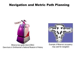
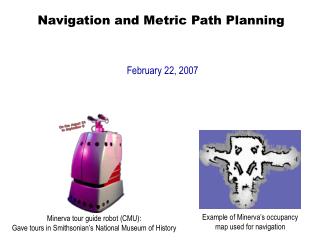
Navigation and Metric Path Planning. February 27, 2007. Victoria’s crater, on Mars. http://thetartan.org/2007/2/19/scitech/mars. JPL robot “Opportunity” being driven by autonomous path-planning software. Regular Grids / Occupancy Grids. Superimposes a 2D Cartesian grid on the world space

E N D
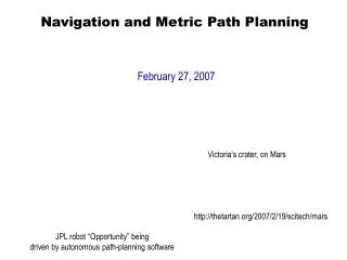
Navigation and Metric Path Planning February 27, 2007 Victoria’s crater, on Mars http://thetartan.org/2007/2/19/scitech/mars JPL robot “Opportunity” being driven by autonomous path-planning software
Regular Grids / Occupancy Grids • Superimposes a 2D Cartesian grid on the world space • If there is any object in the area contained by a grid element, that element is marked as occupied • Center of each element in grid becomes a node, leading to highly connected graph • Grids are either considered 4-connected or 8-connected
Disadvantages of Regular Grids • Digitization bias: • If object falls into even small portion of grid element, the whole element is marked as occupied • Leads to wasted space • Solution: use fine-grained grids (4-6 inches) • But, this leads to high storage cost and high # nodes for path planner to consider • Partial solution to wasted space: Quadtrees
Quadtrees • Representation starts with large area (e.g., 8x8 inches) • If object falls into part of grid, but not all of grid, space is subdivided into for smaller grids • If object doesn’t fit into sub-element, continue recursive subdivision • 3D version of Quadtree – called an Octree.
Example Quadtree Representation (Not all cells are subdivided as in an actual quadtree representation (too much work for a drawing by hand!, but this gives basic idea)
Graph Based Planners • Finding path between initial node and goal node can be done using graph search algorithms • Graph search algorithms: found in networks, routing problems, etc. • However, many graph search algorithms require visiting each node in graph to determine shortest path • Computationally tractable for sparsely connected graph (e.g., Voronoi diagram) • Computationally expensive for highly connected graph (e.g., regular grid) • Therefore, interest is in “branch and bound” search • Prunes off paths that aren’t optimal • Classic approach: A* search algorithm • Frequently used for holonomic robots
“A” Search Algorithm • “A” search: • Produces optimal path • Starts at initial node and works way to goal node • Generates optimal path incrementally • Each update: considers nodes that could be added to the path, and selects best one • Evaluation function: f(n) = g(n) + h(n) where: f(n) measures how good the move to node n is g(n) measures cost of getting to node n from initial node h(n) is the cheapest cost of getting from n to goal • Problem: assumes you know h(n) for all nodes, which means you have to visit all nodes to recurse in order to find h(n)
A* Search Algorithm • A* (read “A star”) search: • Reduces number of paths to be explored • No need to explore a path if it cannot be a good path • Estimates h(n), even if no actual path available • Use this estimate to prune out paths that cannot be good • A* Evaluation function: f*(n) = g*(n) + h*(n) where: * means these are estimates • In path planning, g*(n) is equivalent to g(n) • How to estimate h(n)?
Estimating h(n) • Must ensure that h*(n) is never greater than h(n) (NOTE: Error in book, page 362) • Admissibility condition: • Must always underestimate remaining cost to reach goal • Easy way to estimate: • Use Euclidian (straight line) distance • Straight line will always be shortest path • Actual path may be longer, but admissibility condition still holds
Example of A* Compute optimal path from A-city to B-city Straight-line distance to B-city from: A-city: 366 B-city: 0 F-city: 176 O-city: 380 P-city: 98 R-city: 193 S-city: 253 T-city: 329 Z-city: 374 O-city 71 151 Z-city 75 S-city F-city A-city 140 99 211 80 118 97 R-city B-city T-city 101 P-city
Method for Example • Expand each node from A-city, computing f*(n) = g*(n) + h*(n) • (Example worked on board)
Pros and Cons of A* Search/Path Planner • Advantage: • Can be used with any Cspace representation that can be transformed into a graph • Limitation: • Hard to use for path planning when there are factors to consider other than distance (e.g., rocky terrain, sand, etc.)
Extension to A* = D* • D*: initially plans path to goal just like A*, but plans a path from every position to the goal in advance • I.e., rather than “single source shortest path” (Dijkstra’s algorithm), • Solve “all pairs shortest path” (e.g., Floyd-Warshall algorithm) • In D*, the estimated distance, h*, is based on traversability • Then, D* continuously replans, by updating map with newly sensed information • Approach: “repair” pre-planned paths based on new information Calculate traversability using stereo cameras; can also manually mark maps
D* Applied Recently to Mars Rover “Opportunity” Rover “Opportunity” Image of Victoria crater, taken by rover “Opportunity” Victoria crater, on Mars
Wavefront-Based Path Planners • Well-suited for grid representations • General idea: consider Cspace to be conductive material with heat radiating out from initial node to goal node • If there is a path, heat will eventually reach goal node • Nice side effect: optimal path from all grid elements to the goal can be computed • Result: map that looks like a potential field
Example of Wavefront Planning Goal Start
Algorithmic approach for Wavefront Planning Part I: Propagate wave from goal to start • Start with binary grid; 0’s represent free space, 1’s represent obstacles • Label goal cell with “2” • Label all 0-valued grid cells adjacent to the “2” cell with “3” • Label all 0-valued grid cells adjacent to the “3” cells with “4” • Continue until wave front reaches the start cell. Part II: Extract path using gradient descent • Given label of start cell as “x”, find neighboring grid cell labeled “x-1”; mark this cell as a waypoint • Then, find neighboring grid cell labeled “x-2”; mark this cell as a waypoint • Continue, until reach cell with value “2” (this is the goal cell) Part III: Smooth path • Iteratively eliminate waypoint i if path from waypoint i-1 to i+1 does not cross through obstacle • Repeat until no other waypoints can be eliminated • Return waypoints as path for robot to follow
Wavefront Propagation Can Handle Different Terrains • Obstacle: zero conductivity • Open space: infinite conductivity • Undesirable terrains (e.g., rocky areas): low conductivity, having effect of a high-cost path • Also: To save processing time, can use dual wavefront propagation, where you propagate from both start and goal locations
Example Using Dual Wavefront Propagation 10 Iterations 30 Iterations
Dual Wavefront Propagation in Progress 50 Iterations 70 Iterations
Dual Wavefront Propagation in Progress (con’t.) 90 Iterations 110 Iterations
Dual Wavefront Propagation in Progress (con’t.) Propagation complete.
Extracted Path Goal position Starting position
Summary of Metric Path Planning • Converts world space to a configuration space • Use obstacle growing to enable representation of robot as a point • Cspace representations exploit interesting geometric properties of the environment • Representations can be converted to graphs • A* works well with Voronoi diagrams, since they produce sparse graphs • Wavefront planners work well with regular grids • Metric path planning tends to be computationally expensive • Limitation of popular path planners: assume holonomic robots
Topological Navigation and Path Planning • Based upon points of interest • E.g., landmarks • Navigation is relational between points of interest • E.g., “Go past the corner and enter the second doorway on the left” • Precise metric information not used • Approaches are usually based upon graph representations
Recall: Difference between Topological and Metric • Qualitative (topological, route): • Quantitative (metric or layout): derived from:
Landmarks • Landmark: • One or more perceptually distinctive features of interest on on object or locale of interest • Examples: corner, doorway, tree, sign, marker • Can be “artificial” or “natural” • Artificial placed for the purpose of aiding navigation • Natural existing features not expressly designed for aiding navigation • Gateways: • Special case of landmark, where robot has opportunity to change its overall direction of navigation • Examples: intersection of hallways
Important Criteria for Landmarks • Must be readily recognizable • Must support the task dependent activity • Must be perceivable from many different viewpoints
Relational Methods • Represent world as graph or network of nodes and edges • Nodes: represent gateways, landmarks, or goals • Edges: represent a navigable path between two nodes; can also have additional information attached (e.g., direction, terrain type, behaviors needed to navigate the path)
Multi-Level Spatial Hierarchy (Byun & Kuipers) • Metric: distances, directions, shapes in coordinate system • Topological: connectivity • Landmark definitions, procedural knowledge for traveling
Distinctive Places • Distinctive place: landmark that robot can detect from nearby region called “neighborhood” • Once robot in the neighborhood, it uses sensors to position itself relative to the landmark • Edge in the relational graph: local control strategy (lcs) • Procedure for getting from current node to next node • When landmark sensed, “hill-climbing” used to desired relative position • Maximum value = distinctive place
Example of Distinctive Place distinctive place (within the corner) neighborhood boundary path of robot as it moves into neighborhood and to the distinctive place Robot moves to distinctive place using sensor-based local control strategy and hill-climbing
Example of Local Control Strategies Basic behavior:follow-hall Releasers:look-for-T, look-for-dead-end, look-for-door, look-for-blue dead end follow-hall, with look-for-T follow-hall, with look-for-dead-end follow-hall with look-for-T Blue door T junction follow-hall, with look-for-door, look-for-blue follow-hall, with look-for-door follow-hall, with look-for-T front door
Distinctive Places: Advantages and Disadvantages • Advantages: • Eliminates concern over navigational errors at each node • Robot can build up metric information over multiple trips, since error will average out • Supports discovery of new landmarks • Disadvantages: • Difficult to find good distinctive places • Either too numerous, and thus not locally unique • Or, too few, and thus hard to find • Difficult to define and learn local control strategies