Download
1 / 52
520 likes | 672 Views
Modeling Metacommunities : A comparison of Markov matrix models and agent-based models with empirical data. Edmund M. Hart and Nicholas J. Gotelli Department of Biology The University of Vermont. Talk Overview. Objective Introduction to coexistence models Model system overview

E N D
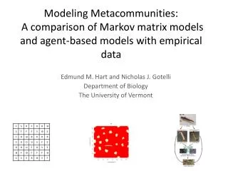
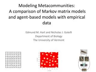
Modeling Metacommunities: A comparison of Markov matrix models and agent-based models with empirical data Edmund M. Hart and Nicholas J. Gotelli Department of Biology The University of Vermont
Talk Overview • Objective • Introduction to coexistence models • Model system overview • Markov matrix model methods • Agent based model (ABM) methods • Comparison of model results and empirical data • Comparison of modeling methods
Objective • To use community assembly rules to construct a Markov matrix model and an ABM to generate models of species coexistence. • Compare two different methods for modeling metacommunities to empirical data to assess their performance. • Can simple rules be used to accurately model real systems?
Classical models and their multispecies expansions (eg Chesson 1994) Lotka-Volterra Competition Model N2 N1
Mechanisms to Enhance Coexistence in Closed Communities • Environmental Complexity Niche dimensionality, Spatial refuges • Multispecies Interactions Indirect effects • Complex Two-Species Interactions Intra-Guild Predation, Ratio of inter to intra specific competition • Neutral models Unstable coexistence and ecological drift
Classical spatial models Levins patch-occupancy metapopulation model All population vital rates are condensed into probability of immigration and extinction
Metacommunity models • Models in spatially homogenous resources • Patch-dynamics • Life history trade-offs, e.g. competition-colonization • Trade-offs allow spatial niche-differences along a single resource niche axis • Neutral models • All species are equivalent, no trade-offs • Differences in community structure come from ecological drift and speciation.
Metacommunity models • Models in spatially heterogenous resources • Species sorting • Local dynamics on a different time scale than regional colonization events • Similar to classical niche-theory, communities are stable and colonization not so frequent that species persist in sinks • Mass effects • A multi-species source sink model, local and regional dynamics on similar time scales • Asymmetric dispersal from spatial storage effects enhances local birth rates
Can we model metacommunity structure using community assembly rules?
A Minimalist Metacommunity P N1 N2
A Minimalist Metacommunity P Top Predator N1 N2 Competing Prey
MetacommunitySpecies Combinations Ѳ N1 N2 P N1N2 N1P N2P N1N2P
Actual data Species occurrence records for tree hole #2 recorded biweekly from 1978-2003(!)
Actual data Toxorhynchitesrutilus P Ochlerotatustriseriatus Aedesalbopictus N1 N2
Stage at time (t) • = Stage at time (t + 1)
“Community” “Patch”
Community Assembly Rules • Single-step assembly & disassembly • Single-step disturbance & community collapse • Species-specific colonization potential • Community persistence (= resistance) • Forbidden Combinations & Competition Rules • Overexploitation & Predation Rules • Miscellaneous Assembly Rules
Competition Assembly Rules • N1 is an inferior competitor to N2 • N1 is a superior colonizer to N2 • N1 N2 is a “forbidden combination” • N1 N2 collapses to N2 or to 0, or adds P • N1 cannot invade in the presence of N2 • N2 can invade in the presence of N1
Predation Assembly Rules • P cannot persist alone • P will coexist with N1 (inferior competitor) • P will overexploit N2 (superior competitor) • N1 can persist with N2 in the presence of P
Miscellaneous Assembly Rules • Disturbances relatively infrequent (p = 0.1) • Colonization potential: N1 > N2 > P • Persistence potential: N1 > PN1 > N2 > PN2 > PN1N2 • Matrix column sums = 1.0
Pattern Oriented Modeling • Use patterns in nature to guide model structure (scale, resolution, etc…) • Use multiple patterns to eliminate certain model versions • Use patterns to guide model parameterization
ABM Assembly Rules • N1 is an inferior competitor to N2 • N1 is a superior colonizer to N2 • N1 N2 is a “forbidden combination” • N1 N2 collapses to N2 or to 0, or adds P • N1 cannot invade in the presence of N2 • N2 can invade in the presence of N1 • P cannot persist alone • P will coexist with N1 (inferior competitor) • P will overexploit N2 (superior competitor) • N1 can persist with N2 in the presence of P • Disturbances relatively infrequent (p = 0.1) • Colonization potential: N1 > N2 > P
Randomly generated metacommunity patches by ABM • 150 x 150 randomly generated • metacommunity, patches are • between 60 and 150 cells, with a • minimum buffer of 15 cells. • Initial state of 100 N1 and N2 and 75 P • all randomly placed on habitat patches. • All models runs had to be 2000 time steps long in order to be analyzed.
ABM community frequency output The average occupancy for all patches of 10 runs of a 25 patch metacommunity for 2000 times-steps
Why the poor fit? – Markov models “Forbidden combinations”, and low predator colonization High colonization and resistance probabilities dictated by assembly rules
Why the poor fit? – ABM Species constantly dispersing from predator free source habitats allowing rapid colonization of habitats, and rare occurence of single species patches Predators disperse after a patch is totally exploited
Metacommunity dynamics of mosquitos Ellis et al found elements of life history trade offs, but also strong correlations between species and habitat, indicating species-sorting Ellis, A. M., L. P. Lounibos, and M. Holyoak. 2006. Evaluating the long-term metacommunity dynamics of tree hole mosquitoes. Ecology 87: 2582-2590.
Concluding thoughts… • Models constructed using simple assembly rules just don’t cut it. • Need to parameretized with actual data or have a more complicated set of assumptions built in. • Using similar assembly rules, Markov models and ABM’s produce different outcomes. • Differences in how space and time are treated • Differences in model assumptions (e.g. immigration) • Given model differences, modelers should choose the right method for their purpose
Acknowledgements Markov matrix modeling Nicholas J. Gotelli– University of Vermont Mosquito data Phil Lounibos – Florida Medical Entomology Lab Alicia Ellis - University of California – Davis Computing resources James Vincent – University of Vermont Vermont Advanced Computing Center