Download

1 / 29
290 likes | 405 Views
Finite Elements. A Theory-lite Intro Jeremy Wendt April 2005. Overview. Numerical Integration Finite Differences Finite Elements Terminology 1D FEM 2D FEM 1D output 2D FEM 2D output Dynamic Problem. Numerical Integration.

E N D
Finite Elements A Theory-lite Intro Jeremy Wendt April 2005 The University of North Carolina – Chapel Hill COMP259-2005
Overview • Numerical Integration • Finite Differences • Finite Elements • Terminology • 1D FEM • 2D FEM 1D output • 2D FEM 2D output • Dynamic Problem The University of North Carolina – Chapel Hill COMP259-2005
Numerical Integration • You’ve already seen simple integration schemes: particle dynamics • In that case, you are trying to solve for position given initial data, a set of forces and masses, etc. • Simple Euler rectangle rule • Midpoint Euler trapezoid rule • Runge-Kutta 4 Simpson’s rule The University of North Carolina – Chapel Hill COMP259-2005
Numerical Integration II • However, those techniques really only work for the simplest of problems • Note that particles were only influenced by a fixed set of forces and not by other particles, etc. • Rigid body dynamics is a step harder, but still quite an easy problem • Calculus shows that you can consider it a particle at it’s center of mass for most calculations The University of North Carolina – Chapel Hill COMP259-2005
Numerical Integration III • Harder problems (where neighborhood must be considered, etc) require numerical solvers • Harder Problems: Heat Equation, Fluid dynamics, Non-rigid bodies, etc. • Solver types: Finite Difference, Finite Volume, Finite Element, Point based (Lagrangian), Hack (Spring-Mass), Extensive Measurement The University of North Carolina – Chapel Hill COMP259-2005
Numerical Integration IV • What I won’t go over at all: • How to solve Systems of Equations • Linear Algebra, MATH 191,192,221,222 The University of North Carolina – Chapel Hill COMP259-2005
Finite Differences • This is probably the easiest solution technique • Usually computed on a fixed width grid • Approximate stencils on the grid with simple differences The University of North Carolina – Chapel Hill COMP259-2005
Finite Differences (Example) • How we can solve Heat Equation on fixed width grid • Derive 2nd derivative stencil on white board • Boundary Conditions • See Numerical Simulation in Fluid Dynamics: A Practical Introduction • By Griebel, Dornseifer and Neunhoeffer The University of North Carolina – Chapel Hill COMP259-2005
Finite Elements Terminology • We want to solve the same problem on a non-regular grid • Draw Grid on Board • Node • Element The University of North Carolina – Chapel Hill COMP259-2005
Problem Statement 1D • STRONG FORM • Given f: OMEGA R1 and constants g and h • Find u: OMEGA R1 such that • uxx + f = 0 • ux(at 0) = h • u(at 1) = g • (Write this on the board) • u – unknown values • f – known values “forces” The University of North Carolina – Chapel Hill COMP259-2005
Problem Statement (cont) • Weak Form (AKA Equation of Virtual Work) • Derived by multiplying both sides by weighting function w and integrating both sides • Remember Integration by parts? • Integral(f*gx) = f*g - Integral(g*fx) The University of North Carolina – Chapel Hill COMP259-2005
Galerkin’s Approximation • Discretize the space • Integrals sums • Weighting Function Choices • Constant (used by radiosity) • Linear (used by Mueller, me (easier, faster)) • Non-Linear (I think this is what Fedkiw uses) The University of North Carolina – Chapel Hill COMP259-2005
Definitions • wh = SUM(cA*NA) • uh = SUM(dA*NA) + g*NA • cA, dA, g – defined on the nodes • cA = 1 (I think) • dA = value of unknown at node • g = bdry condition • NA , uh, wh – defined in whole domain • NA - Shape Functions • wh – weighting function The University of North Carolina – Chapel Hill COMP259-2005
Zoom in • We’ve been considering the whole domain, but the key to FEM is the element • Zoom in to “The Element Point of View” The University of North Carolina – Chapel Hill COMP259-2005
Element Point of View • Don’t construct an NxN matrix, just a matrix for the nodes this element effects (in 1D it’s 2x2) • Integral(NAx*NBx) • Reduces to width*slopeA*slopeB for linear 1D The University of North Carolina – Chapel Hill COMP259-2005
Now for RHS • We are stuck with an integral over varying data (instead of nice constants from before) • Fortunately, these integrals can be solved by hand once and then input into the solver for all future problems (at least for linear shape functions) The University of North Carolina – Chapel Hill COMP259-2005
Change of Variables • Integral(f(y)dy)domain = T = Integral(f(PHI(x))*PHIx*dx)domain = S • Write this on the board so it makes some sense The University of North Carolina – Chapel Hill COMP259-2005
Creating Whole Picture • We have solved these for each element • Individually number each node • Add values from element matrix to corresponding locations in global node matrix The University of North Carolina – Chapel Hill COMP259-2005
Example • Draw even spaced nodes on board • dx = h • Each element matrix = (1/h)*[[1 -1] [-1 1]] • RHS = (h/6)*[[2 1] [1 2]] The University of North Carolina – Chapel Hill COMP259-2005
Show Demo • 1D FEM The University of North Carolina – Chapel Hill COMP259-2005
2D FEM 1D output • Heat equation is an example here • Linear shape functions on triangles Barycentric coordinates • Kappa joins the party • Integral(NAx*Kappa*NBx) • If we assume isotropic material, Kappa = K*I The University of North Carolina – Chapel Hill COMP259-2005
2D Per-Element • This now becomes a 3x3 matrix on both sides • Anyone terribly interested in knowing what it is/how to get it? The University of North Carolina – Chapel Hill COMP259-2005
Demo • 2D FEM - 1D output The University of North Carolina – Chapel Hill COMP259-2005
2D FEM – 2D Out • Deformation in 2D requires 2D output • Need an x and y offset • Doesn’t handle rotation properly • Each element now has a 6x6 matrix associated with it • Equation becomes • Integral(BAT*D*BB) for Stiffness Matrix • BA/B – a matrix containing shape function derivatives • D – A matrix specific to deformation • Contains Lame` Parameters based on Young’s Modulus and Poisson’s Ratio (Anyone interested?) The University of North Carolina – Chapel Hill COMP259-2005
Demo • 2D Deformation The University of North Carolina – Chapel Hill COMP259-2005
Dynamic Version • The stiffness matrix (K) only gives you the final resting position • Kuxx = f • Dynamics is a different equation • Muxx + Cux + Ku = f • K is still stiffness matrix • M = diagonal mass matrix • C = aM + bK (Rayliegh damping) The University of North Carolina – Chapel Hill COMP259-2005
Demo • 2D Dynamic Deformation The University of North Carolina – Chapel Hill COMP259-2005
Good Sources • Papers with a graphics slant: • Matthias Mueller: http://www.matthiasmueller.info/ • Ron Fedkiw (et.al): http://graphics.stanford.edu/~fedkiw/ • Books on FEM and Numerical Methods: • Finite Element Method: Linear Static and Dynamic Finite Element Analysis by Thomas J.R. Hughes • Numerical Simulation in Fluid Dynamics by Griebel, Dornseifer, Neunhoeffer • Computational Fluid Dynamics by T.J. Chung • Classes on PDEs and Numerical Methods/Solutions: • Math 191, 192 (I took from David Adalsteinsson) , 221, 222 (both from Michael Minion) The University of North Carolina – Chapel Hill COMP259-2005
Questions The University of North Carolina – Chapel Hill COMP259-2005