Download
1 / 68
700 likes | 989 Views
Series-Expansion Methods . Agathe Untch e-mail: Agathe.Untch@ecmwf.int (office 011). Acknowledgement This lecture draws heavily on lectures by Mariano Hortal (former Head of the Numerical Aspects Section, ECMWF) and on the excellent textbook

E N D
Series-Expansion Methods Agathe Untch e-mail: Agathe.Untch@ecmwf.int (office 011) Numerical Methods: Series-Expansion Methods
Acknowledgement This lecture draws heavily on lectures by Mariano Hortal (former Head of the Numerical Aspects Section, ECMWF) and on the excellent textbook “Numerical Methods for Wave Equations in Geophysical Fluid Dynamics” by Dale R. Durran (Springer, 1999) Numerical Methods: Series-Expansion Methods
Introduction • The ECMWF model uses series-expansion methods in the horizontal and in the vertical • It is a spectral model in the horizontal with spherical harmonics expansion with triangular truncation. • It uses the spectral transform method in the horizontal with fastFourier transform and Legendre transform. • The grid in physical space is a linearreducedGaussian grid. • In the vertical it has a finite-element scheme with cubic B-spline expansion. • This lecture explains the concept of series-expansion methods (with focus on the spectral method), their numerical implementation, and what the above jargon all means. Numerical Methods: Series-Expansion Methods
Schematic representation of the spectral transform method in the ECMWF model Grid-point space -semi-Lagrangian advection -physical parametrizations -products of terms FFT Inverse FFT Fourier space Fourier space Inverse LT LT Spectral space -horizontal gradients -semi-implicit calculations -horizontal diffusion FFT: Fast Fourier Transform, LT: Legendre Transform Numerical Methods: Series-Expansion Methods
Introduction • Series-expansion methods which are potentially useful in geophysical fluid dynamics are • the spectral method • the pseudo-spectral method • the finite-element method • All these series-expansion methods share a common foundation Numerical Methods: Series-Expansion Methods
Fundamentals of series-expansion methods We demonstrate the fundamentals of series-expansion methods on the following problem for which we seek solutions: Partial differential equation: (with an operator H involving only derivatives in space.) (1) To be solved on the spatial domain S subject to specified initial and boundary conditions. Initial condition: (1a) Boundary conditions: Solution f has to fulfil some specified conditions on the boundary of the domain S. Numerical Methods: Series-Expansion Methods
The set of expansion function should span the L2 space, i.e. a Hilbert space with the inner (or scalar) product of two functions defined as Fundamentals of series-expansion methods (cont) The basic idea of all series-expansion methods is to write the spatial dependence of f as a linear combination of known expansion functions (3) (4) The expansion functions should all satisfy the required boundary conditions. Numerical Methods: Series-Expansion Methods
is only an approximation to the true solution f of the equation (1). The task of solving (1) has been transformed into the problem of finding the unknown coefficients in a way that minimises the error in the approximate solution. Fundamentals of series-expansion methods (cont) Numerically we can’t handle infinite sums. Limit the sum to a finite number of expansion terms N (3a) => Numerical Methods: Series-Expansion Methods
R = amount by which the approximate solution fails to satisfy the governing equation. Fundamentals of series-expansion methods (cont) However, the real error in the approximate solution can’t be determined. A more practical way to try and minimise the error is to minimise theresidual R instead: (5) <=> (1) Strategies for minimising the residual R: 1.) minimise the l2-norm of R 2.) collocation strategy 3.) Galerkin approximation (Details on the next slide.) Each of these strategies leads to a system of N coupled ordinary differential equations for the time-dependent coefficients ai(t), i=1,…, N. Numerical Methods: Series-Expansion Methods
Fundamentals of series-expansion methods (cont) Strategies for constraining the size of the residual: 1.) Minimisation of the l2-norm of the residual Compute the ai(t) such as to minimise (6) 2.) Collocation method Constrain the residual by requiring it to be zero at a discrete set of grid points (7) 3.) Galerkin approximation Require R to be orthogonal to each of the expansion functions used in the expansion of f, i.e. the residual depends only on the omitted basis functions. (8) Numerical Methods: Series-Expansion Methods
Fundamentals of series-expansion methods (cont) • Galerkin method and l2-norm minimisation are equivalent when applied to problems of the form given by equation (1). (Durran,1999) • Different series expansion methods use one or more of this strategies to minimise the error • Collocation strategy is used in the pseudo-spectral method • Galerkin and l2-norm minimisation are the basis of the spectral method • Galerkin approximation is used in the finite-element method Numerical Methods: Series-Expansion Methods
=0 (Galerkin approximation) (9) Fundamentals of series-expansion methods (cont) Transform equation (1) into series-expansion form: Start from equation (5) (equivalent to (1)) (5) Take the scalar product of this equation with all the expansion functions and apply the Galerkin approximation: => Numerical Methods: Series-Expansion Methods
such that Compute the coefficients gives the best approximation to Fundamentals of series-expansion methods (cont) Initial state in series-expansion form: (2) Initial condition (10) The same strategies used for constraining the residual R in (5) can be used to minimise the error r in (10). Using the Galerkin method gives for all j=1,…, N. =0 (Galerkin approximation) Numerical Methods: Series-Expansion Methods
Fundamentals of series-expansion methods (cont) Initial state (cont): for all j=1,…, N. for all j=1,…, N. (11) => (11a) Numerical Methods: Series-Expansion Methods
Fundamentals of series-expansion methods (cont) Summary of the initial value problem (1) in series-expansion form Differential equation (1): (9) Initial condition: (11) Boundary conditions: The expansion functions have to satisfy the required conditions on the boundary of the domain S => approximated solution also satisfies these boundary conditions. Numerical Methods: Series-Expansion Methods
Fundamentals of series-expansion methods (cont) What have we gained so far from applying the series-expansion method? Transformed the partial differential equation into ordinary differential equations in time for the expansion coefficients ai(t). Equations look more complicated than in finite-difference discretisation. Main benefit from the series-expansion method comes from choosing the expansion functions judiciously depending on the form and properties of the operator H in equation (1) and on the boundary conditions. For example, if we know the eigenfunctions ei of H, (i.e. ) and we choose these as expansion functions, the problem simplifies to (12) Numerical Methods: Series-Expansion Methods
Fundamentals of series-expansion methods (cont) If the functions ei are orthogonal and normalised functions, i.e. (13) where (14) then the set of coupled equations (12) decouples into N independent ordinary differential equations in t for the expansion coefficients a (15) Can be solved analytically! Numerical Methods: Series-Expansion Methods
The Spectral Method This is a very helpful simplification, because we obtain explicit equations in when the time derivatives are replaced with finite-differences. The feature that distinguishes the spectral method from other series-expansion methods is that the expansion functions form anorthogonal set on the domain S (not necessarily normalised). (16) => the system of equations (9) reduces to (17) In the more general equation (9) matrix W (defined in (11)) introduces a coupling between all the a at the new time level => implicit equations, more costly to solve! Numerical Methods: Series-Expansion Methods
The Spectral Method (cont) Initial condition (11) simplifies to (18) (18a) <=> Where Numerical Methods: Series-Expansion Methods
The Spectral Method (cont) Summary of the original problem (1) in spectral representation Expansion functions: Form an orthogonal set on the domain S (16) Differential equation: (17) Initial condition: (18) Boundary conditions: The expansion functions have to satisfy the required conditions on the boundary of the domain S => approximated solution also satisfies these boundary conditions. Numerical Methods: Series-Expansion Methods
The Spectral Method (cont) The choice of families of orthogonal expansion functions is largely dictated by the geometry of the problem and the boundary conditions. Examples: Rectangular domain with periodic boundary conditions: Fourier series Non-periodic domains: (maybe) Chebyshev polynomials Spherical geometry: spherical harmonics Numerical Methods: Series-Expansion Methods
(19a) (with constant advection velocity u) (domain S) (19b) (initial condition) The Spectral Method (cont) Example 1:One-dimensional linear advection (19c) (periodic boundary condition) In this case the spatial operator H in (1) is Since u is constant, it is easy to find expansion functions that are eigenfunctions to H. => This problem is almost trivial to solve with the spectral method, but is a good case to reveal some of the fundamental strengths and weaknesses of the spectral method. Numerical Methods: Series-Expansion Methods
The Spectral Method (cont) Example 1:One-dimensional linear advection (cont) (20) Fourier functions are eigenfunctions of the derivative operator They are orthogonal: (21) Approximate f as finite series expansion: (22) Insert (22) into (19a) and apply the Galerkin method => system of decoupled eqs (23) Numerical Methods: Series-Expansion Methods
The Spectral Method (cont) Example 1:One-dimensional linear advection (cont) (23) No need to discretise in time, can be solved analytically: In physical space the solution is: (24) This is identical to the analytic solution of the 1d-advection problem with constant u. => Discretisation in space with the spectral method does not introduce any distortion of the solution: no error in phase speed or amplitude of the advected waves, i.e. no numerical dispersion or amplification/damping introduced, not even for the shortest resolved waves! (The centred finite-difference scheme in space introduces dispersion.) Numerical Methods: Series-Expansion Methods
The Spectral Method (cont) Stability: Integration in time by finite-difference (FD) methods when the spectral method is used for the spatial dimensions typically require shorter time steps than with FD methods in space. This is a direct consequence of the spectral method’s ability to correctly represent even the shortest waves. Leapfrog time integration of the 1d linear advection equation is stable if for spectral where for centred 2nd-order FD Higher order centred FD have more restrictive CFLs, and for infinite order FD (as for spectral!) Numerical Methods: Series-Expansion Methods
The Spectral Method (cont) Stability (cont): The reason behind the less restrictive CFL criterion for the centred 2nd-order FD scheme lies the misrepresentation of the shortest waves by the FD scheme: for centred 2nd-order FD The numerical phase speed ck is for spectral (correct value!) The stability criterion of the leapfrog scheme for the 1d linear advection is (FD) (FD) => = (SP) (SP) Numerical Methods: Series-Expansion Methods
(25b) (initial condition) The Spectral Method (cont) Example 2:One-dimensional nonlinear advection (25a) (domain S) (25c) (periodic boundary condition) Approximate f with a finite Fourier series as in (22), insert into (25a) and apply the Galerkin procedure (alternatively, use directly (17)) => (26) Numerical Methods: Series-Expansion Methods
(27) The Spectral Method (cont) Example 2:One-dimensional nonlinear advection (cont) Suppose that u is predicted simultaneously with f and given by the Fourier series Inserting into (30) gives Compact, but costly to evaluate, convolution sum! (27a) <=> Operation count for advancing the solution by one time step is O( (2M+1)2 ). With a finite-difference scheme only O(2M+1) arithmetic operations are required. Numerical Methods: Series-Expansion Methods
The Transform Method (TM) Products of functions are more easily computed in physical space while derivatives are more accurately and cheaply computed in spectral space. It would be nice if we could combine these advantages and get the best of both worlds! For this we need an efficient and accurate way of switching between the two spaces. Such transformations exist: direct/inverseFast Fourier Transforms (FFT) Numerical Methods: Series-Expansion Methods
The Transform Method (cont) The continuous Fourier Transform (FT) Direct Fourier transform (28a) (28b) Inverse Fourier transform For practical applications we need discretised analogues to these continuous Fourier transforms. Numerical Methods: Series-Expansion Methods
The Transform Method (cont) The discrete Fourier Transform The discrete Fourier transform establishes a simple relationship between the 2M+1 expansion coefficients am(t) and 2M+1 independent grid-point values f(xj,,t) at the equidistant points (29) The set of expansion coefficients defines the set of grid-point values through (30b) (discrete inverseFT) Numerical Methods: Series-Expansion Methods
And vice versa: From the set of grid-point values the set of expansion coefficients can be computed from The Transform Method (cont) The discrete Fourier Transform (cont) (30a) (discrete direct FT) Valid because a discrete analogue of the orthogonality of Fourier functions (21) holds: (31) The relations (30a) and (30b) are discretised analogues to the standard FT (28a) and its inverse (28b). (The integral in (28a) is replaced by a finite sum in (30a).) They are known as discrete or finite (direct/inverse) Fourier transform. Numerical Methods: Series-Expansion Methods
At least 2M+1 equidistant grid-points covering the interval are needed if one want to retain in the expansion of f all Fourier modes up to the maximum wave number M. The Transform Method (cont) The discrete Fourier Transform (cont) Remarks: For the discrete Fourier transformations are exact, i.e. you can transform to spectral space and back to grid-point space and exactly recover your original function on the grid. (N: number of grid points.) Numerical Methods: Series-Expansion Methods
The Transform Method (cont) Mathematically equivalent but computationally more efficient finite FTs, so-called Fast Fourier Transforms (FFTs), exist which use only O(NlogN) arithmetic operations to convert a set of N grid-point values into a set of N Fourier coefficients and vice versa. The efficiency of these FFTs is key to the transform method! The basic idea of the transform method is to compute derivatives in spectral space (accurate and cheap!) and products of functions in grid-point space (cheap!) and use the FFTs to swap between these spaces as necessary. Numerical Methods: Series-Expansion Methods
The Transform Method (cont) Back toExample 2:One-dimensional nonlinear advection Instead of evaluating the convolution sum in (27a), use the Transform Method and proceed as follows to evaluate the product term in the non-linear advection equation (25a): (25a) We have both u and f in spectral representation: Step 1 Compute the x-derivative of f by multiplying each am by im Numerical Methods: Series-Expansion Methods
inv. FFT inv. FFT The Transform Method (cont) Step 2 Use inverse FFT to transform both u and to physical space, i.e. compute the values of these two functions at the grid-points Step 3 Compute the product uf’: Step 4 Use direct FFT to transform the product back to spectral space direct FFT Numerical Methods: Series-Expansion Methods
The Transform Method (cont) Question: Is the result for the product obtained with the transform method identical to the product computed by evaluating the convolution sum in (27a)? Answer: The two ways of computing the product give identical results provided aliasing errors are avoided during the computation of the product in physical space. Aliasing errors can be avoided with a sufficiently fine spatial resolution. How fine does it have to be? How many grid points L do we need in physical space to prevent aliasing errors in the product if we have a spectral resolution with maximum wave number M? Numerical Methods: Series-Expansion Methods
aliasing wave number 0 M 2M is the cutoff wave number of the physical grid, where Multiplication of two waves with wave numbers m1 and m2 gives a new wave m1+m2. If m1+m2 > lc , then m1+m2 is aliased into such that appears as the symmetric reflection of m1+m2 about the cut-off wave number lc. The Transform Method (cont) Avoiding aliasing errors: M is the cutoff wave number of the original expansion Question: How large does lc have to be so that no waves are aliased into waves < M? Numerical Methods: Series-Expansion Methods
The Transform Method (cont) A minimum of 2M+1 grid points are needed in physical space to prevent aliasing errors from quadratic terms in the equations if M is the maximum retained wave number in the spectral expansion. Such a grid is referred to as a “quadratic grid”. Quadratic grid = grid with sufficient resolution to avoid aliasing errors from quadratic terms. Lq = 3M+1 Linear grid = grid with L = 2M+1, which ensures exact transformation of the linear terms to spectral space and back (but with aliasing errors from quadratic and higher order terms). Numerical Methods: Series-Expansion Methods
The Transform Method (cont) Viewed differently: Given a resolution in grid-point space with L grid points, the corresponding spectral resolution (maximum wave number) is for the linear grid for the quadratic grid => 1/3 less resolution in spectral space with the quadratic grid than with the linear grid. Using the quadratic grid is equivalent to filtering out the 1/3 largest wave numbers, i.e. the ones that would be contaminated by aliasing errors from the quadratic terms in the equations. Numerical Methods: Series-Expansion Methods
The Spectral Method on the Sphere Spherical Harmonics Expansion Spherical geometry: Use spherical coordinates: longitude latitude Any horizontally varying 2d scalar field can be efficiently represented in spherical geometry by a series of spherical harmonic functions Ym,n: (40) (41) associated Legendre functions Fourier functions Numerical Methods: Series-Expansion Methods
This definition is only valid for ! The Spectral Method on the Sphere Definition of the Spherical Harmonics Spherical harmonics (41) The associated Legendre functionsPm,n are generated from the Legendre Polynomials via the expression (42) Where Pn is the “normal” Legendre polynomial of order n defined by (43) Numerical Methods: Series-Expansion Methods
The Spectral Method on the Sphere Some Spherical Harmonics for n=5 Numerical Methods: Series-Expansion Methods
The Spectral Method on the Sphere Properties of the Spherical Harmonics Spherical harmonics are orthogonal (=> suitable as basis for spectral method!): (44) because the Fourier functions and the Legendre polynomials form orthogonal sets: (45b) (45a) (46) => the expansion coefficients of a real-valued function satisfy (47) Numerical Methods: Series-Expansion Methods
The Spectral Method on the Sphere Properties of the Spherical Harmonics (cont) (48) Eigenfunctions of the derivative operator in longitude. (49) => Not eigenfunctions of the derivative operator in latitude! But derivatives are easy to compute via this recurrence relation. (50) Eigenfunctions of the horizontal Laplace operator! Very important property of the spherical harmonics! • semi-implicit time integration method leads to a decoupled set of equations for the field values at the future time-level => very easy to solve in spectral space! R: radius of the sphere, : horizontal Laplace operator on the sphere. (see next page) Numerical Methods: Series-Expansion Methods
The Spectral Method on the Sphere Properties of the Spherical Harmonics (cont) Horizontal Laplacian operator on the sphere in spherical coordinates: (51) Numerical Methods: Series-Expansion Methods
The Spectral Method on the Sphere Computation of the expansion coefficients (52) (53) Fourier transform followed by Legendre transform Performing only the Fourier transform gives the Fourier coefficients: (54) direct Fourier transform These Fourier coefficients can also be obtained by an inverse Legendre transform of the spectral coefficients am,n: (55) inverse Legendre transform Numerical Methods: Series-Expansion Methods
n n m triangular M M m rhomboidal The Spectral Method on the Sphere Truncating the spherical harmonics expansion For practical applications the infinite series in (52) must be truncated => numerical approximation of the form (56) Examples of truncations: Triangular truncation is isotropic, i.e. gives uniform spatial resolution over the entire surface of the sphere. Best choice of truncation for high resolution models. Numerical Methods: Series-Expansion Methods
The Spectral Method on the Sphere The Gaussian Grid We want to use the transform method to evaluate product terms in the equations in physical space. Need to define the grid in physical space which corresponds to the spherical harmonics expansion and ensures exact numerical transformation between spherical harmonics space and physical space. This grid is called the Gaussian Grid. Spherical harmonics transformation is a Fourier transformation in longitude followed by a Legendre transformation in latitude. => In longitude we use the Fourier grid with L equidistant points along a latitude circle. L=2M+1 for the linear grid L=3M+1 for the quadratic grid Numerical Methods: Series-Expansion Methods
The Spectral Method on the Sphere The Gaussian Grid (cont) In latitude: Legendre transform, i.e. need to compute the following integral numerically with high accuracy (57) Use Gaussian quardature: numerical integration method, invented by C.F. Gauss, that computes the integral of all polynomials of degree 2L-1 or less exactly from just L values of the integrand at special points called Gaussian quadrature points. These quadrature points are the zeros of the Legendre polynomial of degree n (58) How large do we have to chose L? 2L-1 >= largest possible degree of the integrand in (57) (is a polynomial!) Numerical Methods: Series-Expansion Methods