The IIR FILTERs
860 likes | 1.46k Views
These are highly sensitive to coefficients which may affect stability. The magnitude-frequency response of these filters is established while the phase-frequency response is poor. These filters have short time delay and better time response. The IIR FILTERs.

The IIR FILTERs
E N D
Presentation Transcript
These are highly sensitive to coefficients which may affect stability. The magnitude-frequency response of these filters is established while the phase-frequency response is poor. These filters have short time delay and better time response. The IIR FILTERs
FIR have truncated time-response. Thus their frequency response is poor. These can be designed for time-limited as well as frequency-limited response. FIR filters are inherently stable. Can be designed for Linear phase performance. …..contd The FIR filters
Any arbitrary magnitude response can be designed using frequency sampling technique. They are inherently stable. It is the first choice of the designer if the time delay is not important, even though components required are many more times. …..contd Advantages of FIR filters
It is simple to implementation. The finite word length effect is far less severe on frequency performance. Non-causal filters can be designed for the use of mathematical manipulations. To reduce the computation time of convolution the long discrete sequences, FFT algorithms are used. Properties of FIR filters….
FFT can be implemented on hardware as well as on soft-ware. FIR filter are implemented non-recursively. But these can be mathematically expressed recursively. It has no support of analog filters. Computer Aided Designs are used to design such filters. Properties of FIR filters….
The following transfer functions, one is recursive and other is non-recursive. Both yield identical magnitude-frequency response. We Compare their computational and storage requirements. Recursive Transfer function H1(z) = (bo+ b1 z-1 + b2 z-2) / (1+a1 z-1 + a 2 z-2) where [bo b1 b2] = [ 0.4981819 0.9274777 0.4981819] [a1 a2] =[ -0.6744878 - 0.3633482] and Comparison between IIR and FIR by example 10.01.
Non recursive transfer function: where h(0) = h(11) = 0.54603280 x 10⁻² h(1) = h(10) = -0.45068750 x 10⁻¹ h(2) = h(9) = 0.69169420 x 10⁻¹ h(3) = h(8) = -0.55384370 x 10⁻¹ h(4) = h(7) = -0.63428410 x 10⁻¹ h(5) = h(6) = 0.57892400 x 100 Example 10.01 contd…
Thus we see that IIR filter requires far less components and storage space. But since FIR filter coefficients are symmetrical, the later results in efficient implementation. Summary:Computational and storage requirements
Phase Delay: A signal consists of several frequency components. The phase delay is the amount of time delay each individual frequency components of the signal suffer while transmitted through a system. Non linear phase characteristics of a system results in phase distortion at the output due to alteration in the phase relationship of frequency components of the signal during processing. Linear Phase response FIR:Tptime-phase delay and Tg time group delay.
Non linear phase delay is undesirable in hi-fi systems such as video-,bio-, data- transmission etc. Mathematical model of phase delay is: Tp = - ()/ For linear phase response, the following conditions should be satisfied: where and are constants. Phase delay contd.
For a filter of length N, If the symmetry is positive, = 0 and = (N -1)/2; and if the symmetry is negative, = /2 and = (N -2)/2). [Ifeachor,”Digital Signal Procesing”2/e, PH,pp344-348] In the expression
It is the average time delay of the frequency components of the composite signal. Mathematically it is defined as: Tg = -d()/d = “the derivative of phase wrt frequency”. For no phase distortion, the should be a constant. Group Delay
Phase Phase delay Tp = - ()/ Group delay Tg = -d()/d= The phase delay = group delay if / is a constant. Phase delay and Group Delay
Figure below shows the waveform of an amplitude-modulated input and the output generated by an LTI system Phase and Group Delays displayed group phase
Note: The carrier component at the output is delayed by the phase delay. the envelope of the output is delayed by the group delay. It is relative to the waveform of the underlying continuous-time input signal The waveform at the output shows distortion if the group delay is not constant. Phase and Group Delays
If the distortion is unacceptable then a delay equalizer is cascaded to enable the overall group delay nearly linear over the frequency band of interest To keep the magnitude response of the parent system unchanged, the magnitude characteristics of delay equalizer need to be constant over the frequency band of interest. Phase and Group Delays
The transfer function of the filter should be symmetrical. This symmetry can be positive or, negative. The word-length N, can be even or, odd. It returns four cases: Necessary and sufficient condition for a linear phase response filter is:
Odd coefficients: ao= h[(N-1)/2]; a(n) = 2h[(N-1)/2 - n] Two cases for odd word-length
Even coefficients: b(n) = 2h(N/2 – n) Two cases for even word-length
Even image symmetrywith odd and even word length. FD=1/2 1st 3rd
Even length filter (IV) always exhibit zero response at FD= 0.5. FD= 0.5 corresponds to half the sampling frequency. Hence it is not suitable for high pass filters. It has zero response at DC too. Conclusion…1 • Negative symmetry filters (II & IV) introduces a phase shift of in the phase response. • It makes output zero at DC or, zero frequency. • not suitable for low pass filters. • These are useful in design of differentiator and Hilbert transformers as they require radians phase shift.
Type I is the most versatile filter. Conclusion….2
Further note that the phase delay for positive symmetry (I and III) or group delay in all the four filters is expressible in terms of the coefficients of the word length of the filter. And hence can be corrected to give a zero phase or, group delay response. Denoting T to be the sampling period, phase delay Tp For filter I and III, = (N-1)T/2; For filter II and IV, = (N – 1 - )T/2. Conclusion….3 [Ifeachor,”Digital Signal Processing” PH, 2/e, pp.344-348.
1. Filter Specifications: Filter transfer function H(z), Required amplitude and phase responses, acceptable tolerances, sampling frequency and the word length of the input data. Coefficient Calculations: to determine the coefficients of H(z) so as to satisfy the filter specifications. STEPS IN FIR FILTER DESIGN
Realization: Conversion of the transfer function into suitable structure. Analysis of finite word length effects: Error effect of quantization of input signal, Effect of coefficient quantization. Optimization of word-length. Implementation: Producing software codes and/or hardware and performing the actual filtering. STEPS IN FIR FILTER DESIGN….
Pass / Stop band specifications: Magnitude deviation (includes ripple) Pass/Stop band edge frequency (or frequencies in case of band pass/stop filter). Sampling Frequency. Word length of the filter Design specifications
The Window Method, Frequency Sampling Method, Optimal or, Min-max design method. Each method can lead to design of a linear phase FIR filter. The common mathematical model is: Methods of Calculation of FIR Coefficients
A suitable window function w[n] is selected, required word length is calculated. Then it is multiplied with the impulse response of a (ideal) LPF. Thus hw [n] = h[n] w[n] Or, hw [n] = H[F] W[F]. The window method
The spectrum of ideal low pass filter have a jump discontinuity at F = Fc. But the windowed spectrum shows over-shoot, ripple and a finite transition width but no abrupt jump. The window method….
It’s normalized signal magnitude at F = Fc is 0.5. It corresponds to attenuation of -6 dB. The ripple in pass band and over-shoot is attributed to Gibb’s phenomena; 9% minimum. The side-lobs produces the ripple in pass band and stop band. The ripples in pass band and stop band have odd symmetry. Window method contd…
The transition width is due to main lob. Wider the main lob, wider is the transit band. Wider is the window width, smaller is the width of main-lob. Number of minima and maxima in the pass band and stop band are decided by N. Unlike in Tchebyshev Filters, the peaks here have different heights, maximum near band edges, decaying thereafter. Window method contd…
Note that number of samples equal maxima and minima of a rectangular window in pass- and stop band. The peak occurs near band edges. Maxima-Minima
This window has two properties: maximum number of alternating maxima and minima and their peaks follow the attenuation at the rate of –6.02dB per octave or, equivalent -20dB/dec. Mathematical model of different type windows follows. Rectangular Window
Window Representation Expression Rectangular wR[n] 1 Bartlett wT[n] 1 – {2|n| / (N-1)} Von Hann whn [n] 0.50 + 0.50 cos{2n/(N-1)} Hamming whm [n] 0.54 + 0.46 cos{2n/(N-1)} Blackman wb [n] 0.42 +0.50 cos{2n/(N-1)} +0.08 cos{4n/(N-1)} Kaiser wK[n,] Io(x1)/Io(x2); ratio of modified bessel function of order zero; where x1=({1 – 4[n/(N-1)]2}); and x2= () Mathematic Models Of Different Type Of Windows
We now examine the characteristics of various other type of windows and compare their performances for N=21and N=51. Before that note various nomeclatures. Characteristics of Windows
GP / GS = Peak Gain of main-lob /side-lobe dB ASL = Side-lobe attenuation = (GP /GS) dB. WM = Half-width of main-lobe W6 /W3 = - 6 dB / -3dB half-width DS = stop-band attenuation dB/dec. FWS = C/N where C= constant of filter. WS = Half width in main-lobe to reach the peak level of first side lob. Aws= Peak side-lobe attenuation in dB AWP = Pass band attenuation in dB Mathematical representation:Nomenclatures
Note: The widths; WM, WS, W6, W3; must be normalized by the window length N. Empirical Values for Kaiser Window depends on the value of defined as: GP = |sinc(j)| / Io(); ASL = Sinh()/0.22; WM = (1+2); W 6 = (0.661+2)
Specify the desired frequency response of the filter Hd(). Obtain the impulse response hD [n] of the desired filter by inverse Fourier transform. Select a window which satisfies the pass-band attenuation specification. PROCEDURE OF CALCULATING FILTER COEFFICIENTS USING WINDOW
Determine the number of coefficients using the appropriate relationship between the filter length and the transition width f expressed as a fraction of the sampling frequency. Obtain the values of w[n] for the chosen window function and that of the actual FIR coefficients h[n] and multiplying them. Plot the response and verify the compliance of specifications. PROCEDURE OF CALCULATING FILTER COEFFICIENTS USING WINDOW…
Summery of ideal impulse response of standard frequency selective filters Note: fc, f1 and f2 are the normalized edge frequencies. N is the length of the filter [Ifeachor: p.353]
The TF of a filter is an even symmetric function. It is an ideal transfer function. It has a linear phase response. Theoretical value of n . But for an FIR filter, n should be finite. With finite n, the response will have ripples. The response will also have at least 9% overs-hoots near critical frequencies, Gibbs Phenomena. Remarks:
If the n in truncated range is increased, ripple is reduced so also the overshoot, upto 9%. Increased n means increase in number of coefficients. Ideal truncation is equivalent to convolving an ideal filter hD having frequency response sinc() with rectangular frequency window, W(). It is equivalent to multiplication in time domain. Remarks:
convolution of an ideal filter with a sinc window function. Peak side lob attenuation
Note: All widths; WM, WS, W6, W3; must be normalized by the window length N. Empirical Values for Kaiser Window depends on the value of defined as: GP = |sinc(j)| / Io(); ASL = Sinh()/0.22; WM = (1+2); W 6 = (0.661+2)
Soln: Meaning of given specifications are: Sampling frequency fs = 8000 Hz. Pass band edge frequency: fc =1500/8000 Transition width f = 500/8000. Stop-band attenuation AWS= > 50 dB Example:Design a low-pass FIR filter to meet the following specs:Pass band edge frequency: 1500 HzTransition width: 500 Hz.Stop-band attenuation AWS= > 50 dBSampling frequency fs = 8000 Hz.
The filter function is HD ()= 2fc sinc(nc). Because of stop-band attenuation characteristics, either of the Hamming, Blackman or, Kaiser windows can be used. We use Hamming window: whm[n] =0.54 + 0.46 cos{2n/(N-1)} Design considerations contd…
f = transition band width/sampling frequency = 0.5/8 =0.0625 = 3.3/N. Thus N = 52.8 53 i.e. for symmetrical window –26 n 26. fc’ = fc + f/2 = (1500+ 250)/8000 = 0.21875. Calculate values of hD [n] and whm[n] for –26 n 26 Add 26 to each index so that the indices range from 0 to 52. Plot the response of the design and verify the specifications. Design considerations contd…