Download
1 / 1
10 likes | 166 Views
Uncertainties in Eddy Covariance fluxes due to post-field data processing: a multi-site, full factorial analysis. SIMONE SABBATINI 1,* , GERARDO FRATINI 2 , NICOLA ARRIGA 1 , DARIO PAPALE 1

E N D
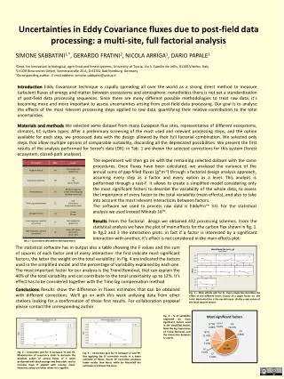
Uncertainties in Eddy Covariance fluxes due to post-field data processing: a multi-site, full factorial analysis SIMONE SABBATINI1,*, GERARDO FRATINI2, NICOLA ARRIGA1, DARIO PAPALE1 1Dept. for Innovation in biological, agro-food and forest systems, University of Tuscia, Via S. Camillo de Lellis, 01100 Viterbo, Italy 2LI-COR Biosciences GmbH, Siemensstraße 25 A, D-61352 Bad Homburg, Germany *Corresponding author. E-mail address: simone.sabbatini@unitus.it IntroductionEddy Covariance technique is rapidly spreading all over the world as a strong direct method to measure turbulent fluxes of energy and matter between ecosystems and atmosphere: nonetheless there is not yet a standardization of post-field data processing sequences. Since there are many different possible methodologies to treat raw data, it’s becoming more and more important to assess uncertainties arising from post-field data processing. Our goal is to analyse the effects of the most relevant processing steps applied to raw data, quantifying their relative contribution to the total uncertainties. Materials and methods We selected some dataset from many European flux sites, representative of different ecosystems, climates, EC system types. After a preliminary screening of the most used and relevant processing steps, and the option available for each step, we processed data with the design allowed by their full factorial combination. We selected only steps that allow multiple options of comparable suitability, discarding all the deprecated possibilities. We present the first results of the analysis performed for Soroe’s data (DK): in Tab. 1 are shown the selected corrections for this system (forest ecosystem, closed-path analyser). The experiment will then go on with the remaining selected dataset with the same procedures. Once fluxes have been calculated, we analysedthe variance of the annual sums of gap-filled fluxes (g*m-2) through a factorial design analysis approach, assuming every step as a factor and every option as a level. This analysis is performed through a test-F. It allows to create a simplified model considering only the most significant factors to describe the variability of the whole data; to assess the importance of every factor to the total variability (main effects), and also to take into account the most relevant interactions between factors. The software we used to process raw data is EddyPro™ 3.0. For the statistical analysis we used instead Minitab 16™. Results From the factorial design we obtained 432 processing schemes. From the statistical analysis we have the plot of main effects for the carbon flux shown in fig. 1. In fig.2 and 3 the interaction plots: in fact if a factor is interested by a significant interaction with another, it’s effect is not considered in the main effects plot. Tab 1 – Corrections selected for the experiment The statistical software has in output also a table showing the F values and the sum of squares of each factor and of every interaction: the first indicate most significant factors, the latter the weight on the total variability. In Fig. 4 are indicated the factors used in the simplified model and the percentage of variability explained by each one. The most important factor for our analysis is the Trend Removal, that can explain the 40% of the total variability and can contribute to the total uncertainty up to 12%. It’s effect has to be considered together with the Time lag compensation method. Conclusions Results show the difference in fluxes estimates that can be obtained with different corrections. We’ll go on with this work anilysing data from other stations looking for a confirmation of those first results. For collaboration proposal please contact the corresponding author. Fig. 1 – Main effects plot for Fc. Every single box describes the effect of the different levels (x-axis) of a single factor on the total. Horizontal line is the overall mean. On the y-axis values of the least squares means. Fig. 4 – % of variability explained by most significant factors used in the simplified model. Note the big importance of Trend Removal, and the interaction between Tr and TL. Fig. 2 – Interaction plot for Fc between TL and TR. Maximization of covariance tends to decrease the absolute values of annual fluxes of C when performed with block avarage and linear detr. and to increase them if applied with running mean. However, values are lower when rm is applied. Fig. 3 – Interaction plot for Fc between LF and HF. Not applying the LF correction results in a lower estimate of fluxes. Ibrom HF correction produces lower results than Horst, while for Moncrieff the estimates are almost the same.