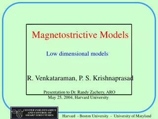
Magnetostrictive Models
Magnetostrictive Models. Low dimensional models. R. Venkataraman, P. S. Krishnaprasad. Presentation to Dr. Randy Zachery, ARO May 25, 2004, Harvard University. Magnetostrictive models. Experimental data from actuators. validation. validation. model. model.


Magnetostrictive Models
E N D
Presentation Transcript
Magnetostrictive Models Low dimensional models R. Venkataraman, P. S. Krishnaprasad Presentation to Dr. Randy Zachery, ARO May 25, 2004, Harvard University
Magnetostrictive models Experimental data from actuators validation validation model model • coupled ODE’s or integro- • differential equations • representing magnetic and • mechanical equilibrium. • material properties appear • through constitutive equations. • eddy-current losses modeled • via a resistance. • coupled PDE’s representing • magnetic and mechanical • dynamic equilibrium. • material properties appear • through shape of potential • functions. • eddy-current losses modeled • via Maxwell’s equations. Micromagnetic model Low-dimensional models model simulation
Derivation of the bulk magnetostriction model. Parameter estimation algorithm. Validation of the model. Discussion of results. Current and future directions. Organization of the talk
W.F. Brown derived expressions for work done by a battery in changing the magnetization of a magneto-elastic body. The body was considered to be a continuum. Jiles and Atherton postulated expressions for magnetic hysteresis losses in a ferromagnet. This lead to an ODE with 5 parameters for the evolution of the average magnetization in a thin ferromagnetic rod. Sablik and Jiles extended this result to a quasi-static magnetostriction model. Hom, Shankar et al. have a model for electrostriction that includes inertial effects. But hysteresis was not modeled. Our Work • Our model takes account of ferromagnetic hysteresis, magnetostriction, inertial effects, mechanical damping and eddy-current effects. It is low-dimensional with 4 continuous states and 12 parameters. • We proposed parameter estimation algorithms that are easy to implement. • We have experimentally verified the structure of our model. • Current work involves inverting the hysteresis nonlinearity and design of a robust controller. Low Dimensional Magnetostrictive Models Background
Langevin’s theory of Paramagnetism Consider a collection of N atomic magnetic moments under the influence of an external magnetic field . Then the average magnetic moment of the ensemble is given by: Weiss’ theory of Ferromagnetism Weiss postulated that an additional “molecular field” experienced by an individual moment in an ideal ferromagnet, where is the average magnetic moment of the ferromagnet. Suppose an external field is applied in the direction of . Then the magnitude of is given by: Weiss considered an ideal ferromagnet without losses. In particular, the curve in the plane is anhysteretic. Derivation of the bulk magnetostriction model
Derivation of the bulk magnetostriction model The anhysteretic magnetization curve
Jiles and Atherton’s assumptions for a lossy ferromagnet • The average magnetization is composed of reversible and irreversible components: • The losses during a magnetization process occur due to the change in the irreversible component: where and are constants with • and . • The reversible and irreversible magnetizations are related to the anhysteretic magnetization as: . • Further and if and Change in kinetic energy Change in internal energy losses Change in external input Derivation of the bulk magnetostriction model Principle of conservation of energy
Derivation of the bulk magnetostriction model W. F. Brown’s expression for work done by the battery where F is the external force, x is the displacement of the tip of the actuator, H is the average external magnetic field, and M is the average magnetization in the actuator. Adding the integral of any perfect differential over a cycle does not change the value on the left hand side. Expressions for some of the energy terms : Magnetoelastic energy density (following Landau) = Elastic energy = ; Kinetic energy =
The bulk magnetostriction model and and otherwise The model equations Magnetic dynamic equilibrium equations Mechanical dynamic equilibrium equation
The bulk magnetostriction model Schematic diagram of the bulk magnetostriction model with eddy current effects included Eddy currents losses are modeled by a resistor in parallel Voltage source displacement output Rate-independent hysteresis operator Mechanical system transfer function
The bulk magnetostriction model Analytical result Theorem : Consider the system of equations (1 - 6). Suppose the matrix A = has eigenvalues with negative real parts and the parameters satisfy conditions (7 - 9). Suppose the input is given by and the initial state is at the origin. Then there exists a such that if then the limit set of the solution trajectory is a periodic orbit. Sufficient condition on parameters where
Parameter Estimation - electrical circuit parameter (includes lead resistance of the magnetizing coil). - eddy current parameter. - magnetic parameters not pertaining to hysteresis. - magnetic hysteresis pertaining to hysteresis. - mechanical dynamic losses parameter. - inertia parameter. - elasticity parameter. - prestress parameter. Three step algorithm for parameter identification Step 1 : Apply a sinusoidal current input of a very low frequency (0.5 Hz) and measure the voltage and displacement of the actuator as a function of time. This leads to the identification of . Repeat the same experiment, for higher frequencies (200Hz, 350 Hz, 500Hz). This leads to identification of . Step 2 : Obtain the anhysteretic displacement curve of the actuator. This leads to the identification of . Step 3 : Apply a swept sine wave current signal to the actuator and record the displacement versus the frequency. This leads to the identification of . The parameters to be found are :
Parameter Estimation Result of parameter estimation Parameter Value (in CGS units) Result of step 2 : Input current waveform Output displacement versus current
Experiment versus Simulation 100 Hz 50 Hz 100 Hz 50 Hz 80 microns 120 microns -1.5 1.5 60 microns 80 microns 1.5 -1.5 Amps Amps -1.5 1.5 -1.5 1.5 Amps Amps 240 Hz 480 Hz 50 microns 500 Hz 200 Hz 45 microns 100 microns 45 microns 1.5 -1.5 -1.5 1.5 Frequency(Hz) Peak-Peak current (A) Peak-Peak displacement ( m) Amps Amps 0.25 2.5 53 1 2.5 53 10 2.5 54 50 2.5 54 100 2.5 51 200 2.5 58 350 2.5 66 500 2.3 44 1.5 -1.5 -1.5 1.5 Amps Amps Frequency(Hz) Peak-Peak current (A) Peak-Peak displacement ( m) 1 2.13 71 10 2.26 71 50 2.17 63 100 2.22 54 150 2.19 50 200 2.28 42 350 2.11 54 500 2.39 45
Validation of the structure of the model Original goal :Trajectory tracking by means of an non-identifier based adaptive controller. Why adaptive control? Reasons :(1) Transient effects are unmodeled in our model. (2) System parameters may change with time due to heating heating etc. Basic idea of universal adaptive stabilization : are unknown and and Then Suppose Therefore is monotonically increasing as Hence long as Hence for decays exponentially and
Validation of the structure of the model for almost all and all (1) (4) and known (3) and all for almost all some scalars and Universal Adaptive Stabilization result for relative degree one systems. Consider a class of nonlinearly-perturbed, single input, single output, linear systems with nonlinear actuator characteristics : Assumptions: (2) The linear system is minimum phase. is a Caratheodory function and has the property that for some scalar is a Caratheodory and has the property that, for some scalar continuous function (5) There exists a map satisfying the condition below and such that condition below and such that every actuator characteristic is contained in the graph of and every in the following sense: with where denotes the restriction of to to compact intervals of with the property that, for is a continuous map from
Validation of the structure of the model Universal Adaptive Stabilization (contd.) The class of reference signals is the Sobolev space with norm Adaptive Strategy (assuming ) : Theorem (Ryan) : Let be a maximal solution of the initial value problem. Then 1. is bounded. 2. 3. exists and is finite. 4.
Validation of the structure of the model Morse-Ryan controller design for relative degree 2 systems Simulation example for Morse-Ryan controller Reference and output trajectories Input non-linearity Gain evolution
Validation of the structure of the model Experimental Setup :
Validation of the structure of the model microns microns microns microns 0 seconds 10 0 seconds 0.4 0 seconds 0.5 0 seconds 0.05 amps amps 0 10 0.05 0 seconds seconds Result of trajectory-tracking experiment Reference (sinusoids) vs. actual displacements Control current amps amps 0.4 0.1 0 0 seconds seconds 1 Hz 500 Hz 50 Hz 200 Hz
Discussion of Results 1. We derived a low dimensional model for a thin magnetostrictive actuator that is phenomenology based and models the magneto-elastic effect; ferromagnetic hysteresis; inertial effects; eddy current effects; and losses due to mechanical motion. The model has 12 parameters, 4 continuous states and can be thought to be composed of magnetic and mechanical sub-systems that are coupled. 2. Analytically we showed that for initial conditions at the origin and periodic inputs, the system equations have a unique solution trajectory that is asympotically periodic. This models experimentally observed phenomena. 3. We have proposed a simple parameter estimation algorithm and estimated the parameters for a commercially available actuator. Simulation results show trajectories that are comparable to the actual. There are some differences in the size of the peak-peak displacement predicted by the simulation and actual results. In particular, the predicted peak-peak displacement is larger than the actual for low frequencies while it is smaller than the actual for high frequencies. This can be explained by an eddy-current resistance value that is slightly smaller than the estimated value. 4. We have also validated the structure of the model by designing a trajectory tracking control-law for relative degree 2 systems with input non-linearity. The closed loop system remained stable for all frequencies from 0 to 750 Hz, thus showing that our model structure is correct.
Current Work and Future Directions 1. The Preisach operator is Lipschitz continuous and its definition can be extended to the space of functions over the real line that are bounded with integrable derivatives over compact intervals. 2. The Preisach operator is rate-independent and models properties that are observed in bulk ferromagnetic hysteresis like minor-loop closure and saturation. 3. It is invertible in the space of functions defined in 1, under some mild conditions on the measure Drawback of the present model : The rate-independent nonlinearity is defined only for periodic signals. Therefore it is unsuitable for the development of a controller. Solution : Replace the rate-independent nonlinearity by a moving Preisach operator, that is defined as follows : where for continuous inputs is defined as for where is a partition such that is monotonic in each sub-interval. Facts about the Preisach operator:
Current Work and Future Directions Current Work 1. We are currently working on an algorithm for the inversion of the Preisach operator, so that we can approximately linearize the rate-independent nonlinearity. 2. Once this is achieved, we can utilize methods from robust control of linear systems for controller design. Future Directions While designing complex magnetostrictive systems, one can obtain low dimensional models from the numerical results obtained from PDE model. This will enable us to short circuit the implementation step and design controllers without actual experimental data.