Chapter 21. Perfect Competition
Chapter 21. Perfect Competition. What is it? Firm behavior Short run Long run. Perfect Competition. many firms, many buyers identical product easy entry/exit for the market prices known existing firms have no advantage. examples. wheat farming dry cleaning.

Chapter 21. Perfect Competition
E N D
Presentation Transcript
Chapter 21. Perfect Competition • What is it? • Firm behavior • Short run • Long run
Perfect Competition • many firms, many buyers • identical product • easy entry/exit for the market • prices known • existing firms have no advantage
examples • wheat farming • dry cleaning
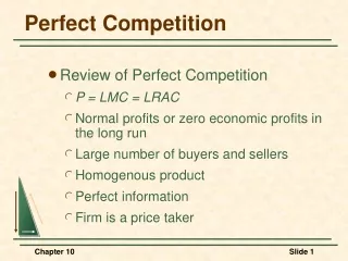
perfectly competitive market • A market with many sellers and • buyers of a homogeneous product • and no barriers to entry. • price taker • A buyer or seller that takes the market price as given.
Here are the five features of a perfectly competitive market: 1 There are many sellers. 2 There are many buyers. 3 The product is homogeneous. 4 There are no barriers to market entry. 5 Both buyers and sellers are price takers.
PREVIEW OF THE FOUR MARKET STRUCTURES • firm-specific demand curve • A curve showing the relationship • between the price charged by a • specific firm and the quantity the firm can sell.
PREVIEW OF THE FOUR MARKET STRUCTURES FIGURE 9.1 Monopoly versus Perfect Competition In Panel A, the demand curve facing a monopolist is the market demand curve. In Panel B, a perfectly competitive firm takes the market price as given, so the firm-specific demand curve is horizontal. The firm can sell all it wants at the market price, but would sell nothing if it charged a higher price.
THE FIRM’S SHORT-RUN OUTPUT DECISION • The Total Approach: Computing Total Revenue and Total Cost
Firm Behavior • maximize profits • TR > TC • economic profits • TR = TC • normal profits
Firm is price taker • cannot influence price • take price as given, choose Q • firm demand is perfectly elastic • horizontal line • MR = P • firm sells all it wants at price, P
Profit maximizing • firm chooses Q to max profits • where TR - TC is largest -- where MR = MC • why MR = MC? • MR > MC -- output adding to profit • MR < MC -- output taking away from profit
P S $8 D Q (cans/day) 100 Market for syrup (all firms)
P MC Q (cans/day) 10 Firm’s demand, cost curve D = MR = P $8
firm is price taker • what if price too low to earn profit? • economic loss • will firm exit?
costs & exit • firm will stay, in SR, if • P > AVC • why? • if firm exits, loses TFC • if P = AVC -- loss from staying = loss from exit
SR equilibrium • two cases • economic profit • economic loss
THE FIRM’S SHORT-RUN OUTPUT DECISION • The Total Approach: Computing Total Revenue and Total Cost ► FIGURE 9.2 Using the Total Approach to Choose an Output Level Economic profit is shown by the vertical distance between the total-revenue curve and the total-cost curve. To maximize profit, the firm chooses the quantity of output that generates the largest vertical difference between the two curves.
THE FIRM’S SHORT-RUN OUTPUT DECISION • The Marginal Approach M A R G I N A L P R I N C I P L E Increase the level of an activity as long as its marginal benefit exceeds its marginal cost. Choose the level at which the marginal benefit equals the marginal cost. • marginal revenue • The change in total revenue from • selling one more unit of output. marginal revenue = price To maximize profit, produce the quantity where price = marginal cost
THE FIRM’S SHORT-RUN OUTPUT DECISION • The Marginal Approach FIGURE 9.3 The Marginal Approach to Picking an Output Level A perfectly competitive firm takes the market price as given, so the marginal benefit, or marginal revenue, equals the price. Using the marginal principle, the typical firm will maximize profit at point a, where the $12 market price equals the marginal cost. Economic profit equals the difference between the price and the average cost ($4.125 = $12 – $7.875) times the quantity produced (eight shirts per minute), or $33 per minute.
THE FIRM’S SHORT-RUN OUTPUT DECISION • Economic Profit and the Break-Even Price economic profit = (price − average cost) × quantity produced • break-even price • The price at which economic profit is • zero; price equals average total cost.
THE FIRM’S SHUT-DOWN DECISION • Total Revenue, Variable Cost, and the Shut-Down Decision operate if total revenue > variable cost shut down if total revenue < variable cost
THE FIRM’S SHUT-DOWN DECISION • Total Revenue, Variable Cost, and the Shut-Down Decision ► FIGURE 9.4 The Shut-Down Decision and the Shut-Down Price When the price is $4, marginal revenue equals marginal cost at four shirts (point a). At this quantity, average cost is $7.50, so the firm loses $3.50 on each shirt, for a total loss of $14. Total revenue is $16 and the variable cost is only $13, so the firm is better off operating at a loss rather than shutting down and losing its fixed cost of $17. The shutdown price, shown by the minimum point of the AVC curve, is $3.00.
THE FIRM’S SHUT-DOWN DECISION • The Shut-Down Price operate if price > average variable cost shut down if price < average variable cost • shut-down price • The price at which the firm is • indifferent between operating and • shutting down; equal to the minimum • average variable cost.
THE FIRM’S SHUT-DOWN DECISION • Fixed Costs and Sunk Costs • sunk cost • A cost that a firm has already paid or • committed to pay, so it cannot be • recovered.
Case 1: economic profit • P = $8, Q = 10 • ATC = $5 • profit = ($8)(10) - ($5)(10) = $30
economic profit P MC ATC $5 Q (cans/day) 10 D = MR = P $8
case 2: economic loss • P = $3, Q = 7 • ATC = $5 • profit = ($3)(7) - ($5)(7) = - $14
economic loss P MC ATC $5 Q (cans/day) 7 D = MR = P $3
12.3 LR Equilibrium • entry & exit of firms • firms earn normal profit • economic profit will be zero
why zero economic profit? • if economic profit > zero • firms enter (S shifts right) • price falls • profit falls to zero
P S S’ $8 $5 D Q (cans/day) 100 120 market for syrup
zero economic profit P MC ATC $5 Q (cans/day) Syrup firm D = MR = P
if economic profit < zero • firms exit (S shifts left) • price rises • profit rises to zero
P S S’’ $5 $3 D Q (cans/day) 120 140 market for syrup
economic loss P MC ATC $5 Q (cans/day) 7 D = MR = P $3
zero economic profit P MC ATC $5 Q (cans/day) Syrup firm D = MR = P
Shifts in market demand • change price in SR • profits or losses • in LR affect exit/entry • return to zero economic profit
Summary • price takers • MR = MC determines equilibrium Q • SR: economic profit or loss • LR: economic profit is zero due to entry/exit