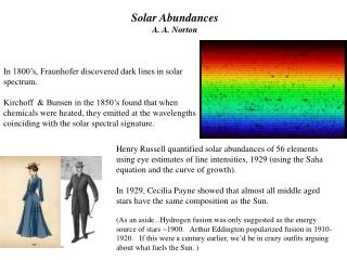
In 1800’s, Fraunhofer discovered dark lines in solar spectrum.

1. Solar Abundances A. A. Norton In 1800’s, Fraunhofer discovered dark lines in solar spectrum. Kirchoff & Bunsen in the 1850’s found that when chemicals were heated, they emitted at the wavelengths coinciding with the solar spectral signature. Henry Russell quantified solar abundances of 56 elements using eye estimates of line intensities, 1929 (using the Saha equation and the curve of growth). In 1929, Cecilia Payne showed that almost all middle aged stars have the same composition as the Sun. (As an aside...Hydrogen fusion was only suggested as the energy source of stars ~1900. Arthur Eddington popularized fusion in 1910-1920. If this were a century earlier, we’d be in crazy outfits arguing about what fuels the Sun. )

2. Nucleosynthesis Big Bang: The observed abundances of H, He and Li are consistent with the photon to baryon ratio assumed in the Big Bang. % by mass: 75 H, 24 He, 0.01 Li Stellar Nucleosynthesis: The burning of the lighter elements - H, He, C, Ne, O, Si, and the CNO cycle. Explosive Nucleosynthesis - Supernova: produces the elements heavier than Fe. (This image is Kepler’s SN 1604 - composite image from Chandra, Spitzer and Hubble.) Cosmic Ray Spallation: Produces light elements 3He, Li, Be and B as a result of cosmic rays impacting the interstellar medium.

3. Units -- The Tower of Babel • Parts per billion by weight (mg of Element/1000 kG) • Mass fractions often quoted X - hydrogen, Y - helium, • Z - heavy elements. Z/X or Y/X values often cited. • Parts per billion by atoms (# atoms of Element/billion atoms) • Solar uses the logarithmic astronomical scale - the # of Hydrogen atoms is assumed to be 1012. • A(H) = log n(H) = 12 dex • A(El) = log (El) = log [n(El)/n(H) ] + 12 • Cosmochemical scale normalizes using the number of Silicon atoms to be 106.

4. Elemental abundances: Solar Photosphere vs Meteorites (CI*) Meteorites are the oldest solar system objects studied in the lab. Can use 87Rb with a 4.8 x 1010 year half life and it’s daughter 87Sr to determine age. *C1 are carbonaceous chondrites that have undergone no or little heating. Values from Asplund, Grevesse, & Sauval, 2005

5. Why abundances are important -- The Standard Solar Model (SSM) Assumptions: 1 solar mass, zero age, initial homogenous chemical composition. Equations: Laws of mass, momentum and energy conservation + energy transport and nuclear reactions. Run time: Model is allowed to evolve to current solar age. Crucial: Results need to match observed solar luminosity, radius and mass. The model should reproduce the observed surface composition.* Abundances: Observed surface values assumed to be the initial solar chemical composition. Excepting -H, Li, Be & B -- affected by nuclear burning and diffusion He which is a free parameter and is not observed in photosphere. Astrophysics Importance: Stellar evolutionary calculations are calibrated with respect to the SSM.

6. Uncertainties/Areas for Improvement Uncertainties: Opacities add 10-20% of the uncertainty in the solar model. The other uncertainties include nuclear reaction cross sections values & the elemental abundances. Areas for Improvement: Add convection, rotation, magnetic fields, account for element diffusion. (Note: Solar Model becomes Non-Standard when these are added.) Along came Helioseismology: The Standard Solar Model was able to reproduce the radius, mass and luminosity to within 0.1% fairly easily which didn’t motivate additional research. Then along came helioseismology and was able to measure oscillation frequencies to within hundreds of a %. The solar model now had a more stringent set of observations to satisfy.

7. What are the current dilemmas in solar abundance research? Helium: Not present in photospheric spectrum and is largely lost by meteorites. Values must be inferred from the corona or the solar wind, but these have large uncertainties (lines formed in non-LTE). Best to use models to get He abundance. Lithium, Beryllium & Boron:Can all be burned by nuclear processes. Li at ~2.5 x 106 K. Be at 3 x 106 K. Li is depleted by 160 whereas Be and B are not depleted. Evidence of the depth of the convection zone! It appears the the solar convection cell has reached deep enough to burn Li, but not Be and B. Neon, Argon:Not present in photospheric spectrum and lost by meteorites so there is uncertainty in the values. Carbon, Nitrogen, Oxygen: These elements are lost by meteorites but are found in the photosphere. Their abundances are dependent upon the treatment of the atmospheric conditions - LTE or non-LTE. Oxygen is also a reference line for Ne and Ar, so if it’s abundance is changed then the abundances of Ne and Ar also scale up or down.

8. The Dilemmascontinued… Gravitational Settling: It is expected that heavier elements should settle to the base of the convection zone and increase the opacity there. Helioseismology shows the sound speed as a function of solar radius to have a ‘bump’. Is this due to gravitational settling? If yes, then why do Be and B not show a deficiency in the photosphere? (Graph from first two years of MDI data.)

9. Solar Abundances in Perspective: The Visible and the Baryonic Bias A NASA pie chart indicating the proportional composition of different energy-density components of the universe, according to CDM model fits. Roughly 95 % is in the exotic forms of dark matter and dark energy. 70 % or more of the universe consists of dark energy, about which we know next to nothing.

10. The Solar Oxygen CrisisSocas-Navarro & Norton, 2007, ApJ, 660, L153 • Oxygen is the 3rd most abundant element in the universe. • Oxygen was not created in the Big Bang. • In stars with M ≥ 4Msun, O is created in Carbon burning process. • If M ≥ 8Msun, O is created in Neon burning process. • CNO-II cycle in massive stars creates O.

11. http://www.webelements.com Universe Sun Elemental abundances in the Universe, the Sun and the Earth’s Crust. By mass-Hydrogen 73.9% Helium 24% Oxygen 1% Earth’s Crust

12. Solar Values of log O (dex) Stellar Values • *A change from 8.93 to 8.63 is a factor of 2 in number densities: ~800 to 400 ppm. • * Lower solar value fits better within galactic environment. • * Lower value ruins agreement between solar interior models and helioseismic results.

13. Spectro-Polarimeter for Infrared and Optical Regions (SPINOR) - Example of Data • Allows simultaneous observations of multiple lines anywhere in the wavelength range 0.4 to 1.6 microns. • Utilizes the adaptive optics system. • Data from 2004: Rows are Stokes I,Q,U,V, and columns are (left to right): Ca II 849.8 nm, Ca II 854.2 nm, and He I 1083.0 nm.

14. Inversion Codes: Often use a least-squares fitting based on the ME solution of the Unno-Rachkovsky equations of a plane-parallel magnetized radiative transfer of the Stokes line profiles (Skumanich and Lites, 1987). Inputs describing the atomic transition of the spectral line are needed. The inversion code fits nine free parameters: the line center, the Doppler width, the damping coefficient, the line to continuum opacity ratio, the slope of the line source function with optical depth, the fill fraction, the magnitude of the magnetic field, the inclination and the azimuth.

15. A New Approach to Measure the Oxygen Abundance • Obtain spatially resolved (0.7”) spectro-polarimetric observationsin Oct ‘06 of Fe I lines at 6302 A as well as the O I triplet at 7774 A. • Use inversion codes to get vertical stratification of temperature, density, line of sight velocity and magnetic field for each pixel in field of view. • Produce 3D semiempirical model from Fe I lines. pore Temperature (left) Magnetic Flux Density (right)

16. Use O I observations to determine abundance at each pixel. Synthetic O I profiles were computed at levels of 0.1 dex and the 2 vs log O curve was interpolated to find the minimum with ~0.01 dex accuracy. Results: 8.93 dex - LTE 8.63 dex - NLTE (+/- 0.08 dex) Comparisons: Traditional value (1D) = 8.93 dex (Anders & Grevesse 1989) 3D theoretical NLTE simulation = 8.66 dex (Aplund et al. 2004)

17. HELIOSEISMIC CONSEQUENCES • Oxygen provides a lot of opacity around the base of the convection zone. • Lowering the opacity at the base of the CV will increase the region where radiative transport is efficient, thus making the convection zone shallower. • Agreement between solar model and NLTE abundance measurements could be restored if opacity is increased ~10-20% at base of CV. (how? Thermal diffusion? Gravitational settling?) • Basu et al (2007) studied the fine-structure spacings of low degree p modes that probe the solar core. They find the lower abundance values simply aren’t supported. Interior modelers Atmospheric modelers Thanks www.edwebproject.org/

18. CONCLUSIONS There are many unresolved issues regarding solar (& stellar) abundances. Results support downward revision of Oxygen abundance. This lower value wreaks havoc with the impressive agreement between standard solar model and helioseismology. However, spatial variation of abundance not expected and leads us to believe that the atmospheric models are still missing some important physics. It’s not clear how the oxygen abundance dilemma will be resolved, but it presents us with an opportunity to improve our models and general understanding.