Download
1 / 24
250 likes | 494 Views
Ray Tracing. Reading. Required: Watt, sections 1.3-1.4, 12.1-12.5.1. T. Whitted. An improved illumination model for shaded display. Communications of the ACM 23(6), 343-349, 1980. [In the reader.] Further reading:

E N D
Reading • Required: • Watt, sections 1.3-1.4, 12.1-12.5.1. • T. Whitted. An improved illumination model for shaded display. Communications of the ACM 23(6), 343-349, 1980. [In the reader.] • Further reading: • A. Glassner. An Introduction to Ray Tracing. Academic Press, 1989. [In the lab.] • K. Turkowski, “Properties of Surface Normal Transformations,” Graphics Gems, 1990, pp. 539-547. [In the reader.] University of Texas at Austin CS384G - Computer Graphics Fall 2008 Don Fussell 2
Geometric optics • Modern theories of light treat it as both a wave and a particle. • We will take a combined and somewhat simpler view of light – the view of geometric optics. • Here are the rules of geometric optics: • Light is a flow of photons with wavelengths. We'll call these flows “light rays.” • Light rays travel in straight lines in free space. • Light rays do not interfere with each other as they cross. • Light rays obey the laws of reflection and refraction. • Light rays travel form the light sources to the eye, but the physics is invariant under path reversal (reciprocity). University of Texas at Austin CS384G - Computer Graphics Fall 2008 Don Fussell 3
Synthetic pinhole camera • The most common imaging model in graphics is the synthetic pinhole camera: light rays are collected through an infinitesimally small hole and recorded on an image plane. • For convenience, the image plane is usually placed in front of the camera, giving a non-inverted 2D projection (image). • Viewing rays emanate from the center of projection (COP) at the center of the lens (or pinhole). • The image of an object point P is at the intersection of the viewing ray through P and the image plane. University of Texas at Austin CS384G - Computer Graphics Fall 2008 Don Fussell 4
Eye vs. light ray tracing • Where does light begin? • At the light: light ray tracing (a.k.a., forward ray tracing or photon tracing) • At the eye: eye ray tracing (a.k.a., backward ray tracing) • We will generally follow rays from the eye into the scene. University of Texas at Austin CS384G - Computer Graphics Fall 2008 Don Fussell 5
Precursors to ray tracing • Local illumination • Cast one eye ray, then shade according to light • Appel (1968) • Cast one eye ray + one ray to light University of Texas at Austin CS384G - Computer Graphics Fall 2008 Don Fussell 6
Whitted ray-tracing algorithm • In 1980, Turner Whitted introduced ray tracing to the graphics community. • Combines eye ray tracing + rays to light • Recursively traces rays • Algorithm: • For each pixel, trace a primary ray in direction V to the first visible surface. • For each intersection, trace secondary rays: • Shadow rays in directions Li to light sources • Reflected ray in direction R. • Refracted ray or transmitted ray in direction T. University of Texas at Austin CS384G - Computer Graphics Fall 2008 Don Fussell 7
Whitted algorithm (cont'd) Let's look at this in stages: University of Texas at Austin CS384G - Computer Graphics Fall 2008 Don Fussell 8
Shading • A ray is defined by an origin P and a unit direction d and is parameterized by t: • P + td • Let I(P, d) be the intensity seen along that ray. Then: • I(P, d) = Idirect+ Ireflected+ Itransmitted • where • Idirectis computed from the Phong model • Ireflected= krI (Q, R) • Itransmitted= ktI (Q, T) • Typically, we set kr= ks and kt = 1 – ks . University of Texas at Austin CS384G - Computer Graphics Fall 2008 Don Fussell 9
Reflection and transmission • Law of reflection: • i= r • Snell's law of refraction: • i sinI = t sint • where i , t are indices of refraction. University of Texas at Austin CS384G - Computer Graphics Fall 2008 Don Fussell 10
Total Internal Reflection • The equation for the angle of refraction can be computed from Snell's law: • What happens when i > t? • When t is exactly 90°, we say that Ihas achieved the “critical angle” c. • For I > c, no rays are transmitted, and only reflection occurs, a phenomenon known as “total internal reflection” or TIR. University of Texas at Austin CS384G - Computer Graphics Fall 2008 Don Fussell 11
Error in Watt!! • In order to compute the refracted direction, it is useful to compute the cosine of the angle of refraction in terms of the incident angle and the ratio of the indices of refraction. • On page 24 of Watt, he develops a formula for computing this cosine. Notationally, he uses m instead of h for the index of refraction in the text, but uses h in Figure 1.16(!?), and the angle of incidence is f and the angle of refraction is q. • Unfortunately, he makes a grave error in computing cosq. He also has some errors in the figures on the same page. • Consult the errata for important corrections! University of Texas at Austin CS384G - Computer Graphics Fall 2008 Don Fussell 12
Ray-tracing pseudocode We build a ray traced image by casting rays through each of the pixels. functiontraceImage (scene): for each pixel (i,j) in image S = pixelToWorld(i,j) P = COP d = (S- P)/|| S– P|| I(i,j) = traceRay(scene, P, d) end for end function University of Texas at Austin CS384G - Computer Graphics Fall 2008 Don Fussell 13
Ray-tracing pseudocode, cont’d functiontraceRay(scene, P, d): (t, N, mtrl) scene.intersect (P, d) Q ray (P, d) evaluated at t I = shade(q, N, mtrl, scene) R = reflectDirection(N, -d) I I + mtrl.kr traceRay(scene, Q, R) if ray is entering object then n_i = index_of_air n_t = mtrl.index else n_i = mtrl.index n_t = index_of_air if(mtrl.k_t > 0 andnotTIR (n_i, n_t, N, -d)) then T = refractDirection (n_i, n_t, N, -d) I I + mtrl.kt traceRay(scene, Q,T) end if return I end function University of Texas at Austin CS384G - Computer Graphics Fall 2008 Don Fussell 14
Terminating recursion • Q: How do you bottom out of recursive ray tracing? • Possibilities: University of Texas at Austin CS384G - Computer Graphics Fall 2008 Don Fussell 15
Shading pseudocode Next, we need to calculate the color returned by the shade function. functionshade(mtrl, scene, Q, N, d): I mtrl.ke + mtrl. ka * scene->Ia foreach light source do: atten = -> distanceAttenuation(Q) * -> shadowAttenuation(scene, Q) I I + atten*(diffuse term + spec term) end for return I end function University of Texas at Austin CS384G - Computer Graphics Fall 2008 Don Fussell 16
Shadow attenuation • Computing a shadow can be as simple as checking to see if a ray makes it to the light source. • For a point light source: function PointLight::shadowAttenuation(scene, P) d = (.position - P).normalize() (t, N, mtrl) scene.intersect(P,d) Q ray(t) ifQ is before the light source then: atten = 0 else atten = 1 end if return atten end function • Q: What if there are transparent objects along a path to the light source? University of Texas at Austin CS384G - Computer Graphics Fall 2008 Don Fussell 17
Ray-plane intersection • We can write the equation of a plane as: • The coefficients a, b, and c form a vector that is normal to the plane, n = [abc]T. Thus, we can re-write the plane equation as: • We can solve for the intersection parameter (and thus the point): University of Texas at Austin CS384G - Computer Graphics Fall 2008 Don Fussell 18
Ray-triangle intersection • To intersect with a triangle, we first solve for the equation of its supporting plane: • Then, we need to decide if the point is inside or outside of the triangle. • Solution 1: compute barycentric coordinates from 3D points. • What do you do with the barycentric coordinates? University of Texas at Austin CS384G - Computer Graphics Fall 2008 Don Fussell 19
Ray-triangle intersection • Solution 2: project down a dimension and compute barycentric coordinates from 2D points. • Why is solution 2 possible? Why is it legal? Why is it desirable? Which axis should you “project away”? University of Texas at Austin CS384G - Computer Graphics Fall 2008 Don Fussell 20
Interpolating vertex properties • The barycentric coordinates can also be used to interpolate vertex properties such as: • material properties • texture coordinates • normals • For example: • Interpolating normals, known as Phong interpolation, gives triangle meshes a smooth shading appearance. (Note: don’t forget to normalize interpolated normals.) University of Texas at Austin CS384G - Computer Graphics Fall 2008 Don Fussell 21
Epsilons • Due to finite precision arithmetic, we do not always get the exact intersection at a surface. • Q: What kinds of problems might this cause? • Q: How might we resolve this? University of Texas at Austin CS384G - Computer Graphics Fall 2008 Don Fussell 22
Intersecting with xformed geometry • In general, objects will be placed using transformations. What if the object being intersected were transformed by a matrix M? • Apply M-1 to the ray first and intersect in object (local) coordinates! University of Texas at Austin CS384G - Computer Graphics Fall 2008 Don Fussell 23
Intersecting with xformed geometry • The intersected normal is in object (local) coordinates. How do we transform it to world coordinates? University of Texas at Austin CS384G - Computer Graphics Fall 2008 Don Fussell 24