Download
1 / 30
300 likes | 550 Views
Networks in Metabolism and Signaling Edda Klipp Humboldt University Berlin Lecture / WS 2007/08 Petri Nets. Petri Nets: Literature. Petri. Petri Nets Invention. Reminder: Stoichiometry. Stoichiometric matrix. Vector of metabolite concentrations. Vector of reaction rates. Parameter vector.

E N D
Networks in Metabolism and Signaling Edda Klipp Humboldt University BerlinLecture / WS 2007/08Petri Nets
Petri Nets: Literature Petri
Reminder: Stoichiometry Stoichiometric matrix Vector of metabolite concentrations Vector of reaction rates Parameter vector Systems equations in matrix form In steady state: K represents the basis vector for all possible steady state fluxes.
Petri Nets – General Remarks Structural Properties Invariants Dynamical Properties Simulation Petri Nets Models Hypotheses Representation and Generation Interaction Patterns Knowledge/Query Representation
Petri Nets – Definitions Petri nets are bipartitedirectedmulti-graphs, i.e., they consist of - two types of nodes, called places and transitions, and - directed arcs, which are weighted by natural numbers and connect only nodes of different type. node transition e.g. metabolites and reactions
Petri Nets – Definitions Examples for places: passive system elements as conditions, states, or biological species, i.e., chemical compounds as proteins. Examples for transitions: active system elements such as events, or chemical reactions such as activation or deactivation
Petri Nets – Definitions The arcs in the net describe the causal relation between active and passive elements. They are illustrated as arrows. They can be labeled with their weight (if appropriate).
Petri Nets – Definitions A Petri net is a 5-tuple, PN = (P,T,F,W,M0) where: is a finite set of places, is a finite set of transitions, is a set of arcs (flow relations), is a weight function, is the initial marking A Petri net structure N = (P,T,F,W) without any specific initial marking is denoted by N. A Petri net with the given initial marking is denoted by (N,M0).
Tokens as Dynamic Elements Arcs connect an event with its preconditions, which must be fulfilled to trigger this event, and with its postconditions, which will be fulfilled, when the event takes place. The fulfillment of a condition is realized via tokens residing in places. Principally, a place in a discrete net may carry any integer number of tokens, indicating different degrees of fulfillment. If all preplaces of a transition are marked sufficiently (corresponding to the arc weights) with tokens, this transition may fire. If a transition fires, tokens are removed from all its preplaces and added to all its postplaces, each corresponding to the given arc weights.
Tokens as Dynamic Elements In short: transitions fire, when enough tokens are present 3 1 2 2 3 1 2 2 Tokens are removed and add as indicated by arc weights.
Tokens as Dynamic Elements If a condition must be fulfilled, but the firing of an adjacent transition does not remove any tokens from it, these nodes are connected via two converse arcs. Such arcs can be represented by bidirectional arrows and called read arcs. 3 1 e.g. enzyme or activator necessary to convert substrates into their products 2 2 3 1 2 2
Marking of a Petri Net A current distribution of the tokens over all places, usually given as M € N0 , describes a certain system state and is called a marking of the net. Accordingly, the initial marking M0 of a net describes the system state before any transition has fired. 3 1 2 2
Marking of a Petri Net The incidence matrix C of a given Petri net is an (n×m)-matrix (where n denotes the number of places and m the number of transitions). Every matrix entry cijgives the token change on the place pi by the firing of the transition tj . The incidence matrix does not reflect read arcs. Note: similarity to stoichiometric matrix for metabolic networks. 3 1 2 2
Petri Nets – Semantics • Explicit representation of causality relations of events and states • Independent events are concurrent (nebenläufig) • Spatially and temporally non-sequential distributed systems • Hierarchical abstraction levels • System properties, system dynamics, proofs
T-Invariants A t-invariant is defined as a non-zero vector x € M0 , fulfilling C . x = 0. A t-invariant represents a multiset of transitions, which have altogether a zero effect on the marking, i.e., if all of them have fired the required number of times, a given marking is reproduced. The invariant property holds for an arbitrary initial marking. A t-invariant is called realizable, if a marking is reachable, such that all transitions of the t-invariant are able to fire in a suitable partial order. Compare: steady state rates, NK=0
P-Invariants A p-invariant is defined as a non-zero vector y € M0 , fulfilling y . C = 0. A p-invariant characterizes a token conservation rule for a set of places, over which the weighted sum of tokens is constant independently from any firing, i.e., for a p-invariant y and any markings Mi, Mj € N0, which are reachable from M0 by the firing of transitions, it holds y . Mi= y . Mj Compare: conservation relations, GN=0
Reversible Reactions A+B C+D D A C B
Siphons, Traps, Deadlocks and Liveness Siphon – place that marked once, remains so. (Input transition set is included in output set) Trap – place that once sufficiently marked, never loses all tokens. (Output transition set included in input set) Deadlock-free – if for any possible marking there is an enabled transition. Deadlock – no more transition possible. Liveness – from the initial marking is a marking reachable, such that a certain transition is enabled.
a Model of Yeast Pheromone Pathway Pheromone Plasma membrane Ste2 Receptor activation G protein cycle Gbg MAPK scaffold Signaling cascade Fus3 Sst2 Far1Cdc28 Bar1 Ste12 Complex formation Gene expression
Model of Yeast Pheromone Pathway Sackmann et al., 2006
Model of Yeast Pheromone Pathway Sackmann et al., 2006
Reconstructing the regulatory network controlling commitment and sporulation in Physarium polycephalum based on hierachical Petri Net modeling and simulation. Marwan W, et al., 2005, JTB
Glucose consumption and starvation of a Physarum plasmodium represented by a Petri Net. Whether the plasmodium is fed or starved is indicated by a token in the respective place. When a starved plasmodium (a) is supplied with glucose (b), glucose is used up (c) and the plasmodium is fed (the token moves from the Starved place to the Fed place by switching of transition T1 which functions as logic AND). With time, the metabolic energy provided by the added glucose is used up and the plasmodium starves again (d). Putting more than one token (n>1) into the Glucose place, glucose consumption according to the model would proceed by cyclically running n-times through states (b), (c), (d) removing one token from the Glucose place in each cycle, while the two places indicating the mutually exclusive physiological states of the plasmodium, fed or starved, always are marked by a single token only.
Sensory control of sporulation in P. polycephalum represented as a Petri Net derived from physiological experiments with wild-type (a) and as a more detailed model (b), refined by including genes involved in sporulation
Modelling of a time-resolved somatic complementation experiment performed by fusion of two plasmodia carrying mutations at different sites of the sporulation control network: (a) Mutant plasmodia before fusion. The flow of tokens along the sporulation control network depends on the activity of transitions which by themselves are controlled by the cellular concentration of the wild-type gene product. In the α-plasmodium T1α is disabled due to a loss-of-function mutation in Gene 1. In the β-plasmodium T2β is disabled due to a loss-of-function mutation in Gene 2. In the α-plasmodium, a token cannot pass T1α. In the β-plasmodium, a token cannot pass T2β and consequently none of the two plasmodia can sporulate. (b) After fusion of the two plasmodia, their protoplasms and suspended nuclei mix due to the vigorous acto-myosin-powered protoplasmic shuttle streaming. The fluxes of tokens along the signalling pathways superimpose with the fluxes of tokens between the plasmodial halves. Note that the tokens representing the gene products do not enter the sporulation control network, since they are connected to the transitions they regulate via test-arcs. In the example shown, the token which was trapped in P1α before fusion occurred (panel A) has moved in the fused plasmodium (panel B) to P2β via P1β and T1β. It could also have moved through T1α provided this transition became activated by supply of (complementation with) the gene product, which was missing before plasmodial fusion occurred.